Break-even Analysis in ExcelLet's perform break-even analysis in excel!

From a previous article, we’ve learned about break-even analysis.

We’ve learned of its definition, the formulas involved, and its benefits.

Break-even analysis is a useful tool that can help you with business decisions that bring in additional costs.

For example, you want to launch a new product.

With break-even analysis, you can determine how many units you must sell for the revenue to fully cover its cost.

We refer to this point as the break-even point, where you neither lose nor gain money.

Break-even analysis can also help with pricing, making sure that a product’s price can cover all its variable and fixed costs.

We’ve learned that we can compute the break-even point using two formulas.

One formula expresses the break-even point in units.

This is particularly useful for product-related revenue.

Just like launching a new product.

You would want to know how many units of the new product you must sell before you can make a profit out of it.

Here it is in formula form:

Break-even Point = Fixed Cost ÷ (Revenue per unit – Variable Cost per unit)

The other formula determines the revenue level that the activity must reach for it to fully cover its costs

If you are able to reach said revenue level, you won’t be losing any money anymore (though you won’t be making money yet either).

By knowing the break-even point, you can assess whether an activity is feasible or not.

You can also use this variation of the formula for service-related revenue.

Here it is in formula form:

Break-even Point = Fixed Cost ÷ Contribution Margin

Where:

Contribution Margin = (Revenue – Variable Cost) ÷ Revenue

Knowing these formulas is essential if you want to perform break-even analysis on excel.

The components of the break-even formula

Both of the break-even point formulas need three variables in their computations: the variable cost, fixed cost, and revenue.

Let’s have a closer look at these variables:

Variable cost

You may have noticed that some of your business’s expenses change depending on the level of production or sales.

For example, the sales commission you pay your sales employees changes depending on the amount products they sell.

Or that the amount you pay for gas depends on your consumption (and also gas prices).

These expenses that increase or decrease depending on the level of activity are what we call variable costs (or variable expenses).

Here are some common examples of variable costs:

• Sale commission (depends on sales)
• Hourly wage (depends on the number of hours worked)
• Cost of raw materials used in production (depends on the level of production)
• Fuel expense (depends on consumption)
• Supplies expense (depends on consumption)

In break-even analysis, we use the variable cost to determine the contribution margin, either expressed on a per-unit or percentage basis.

You must take note that the total variable cost must be less than revenue.

If variable costs equal revenue, you won’t even have a contribution margin, let alone profit.

No amount of revenue will be able to fully cover both variable and fixed costs as it will all be eaten by variable costs alone.

If variable costs exceed revenue, not only will you not be making any profit, but you’d also be automatically incurring a loss.

You must be mindful of this when you’re pricing a product or service.

Fixed Cost

Fixed costs are expenses that don’t change with the changes in the level of activity.

They don’t change when production or sales go up or down (except in step-cost scenarios).

They generally stay the same no matter the level of activity.

These costs do increase or decrease, but not usually due to changes in the level of activity.

One example is the rent you pay for the space that you’re occupying.

Unless it’s stated in the contract, the amount you pay won’t change if there’s an increase or decrease in sales or production.

That said it can change if modifications to the contract were made and approved (e.g. increase in rent due to inflation).

Here are some of the common examples of fixed cost:

• Salaries
• Rent expense
• Insurance expense
• Retainers’ Fee

The fixed cost is an important figure in break-even analysis as it greatly influences the break-even point.

The lower it is, the lower the break-even point is too.

If an activity has no fixed costs, then the break-even point will be at zero level of activity.

This means that any level of activity will produce a profit (provided that revenue exceeds variable cost).

For example, let’s say a product produces a revenue of $15 per unit. It has a variable cost of $8 and no fixed costs. From the moment you sell even just one unit of this product, you’ll already be making a profit of $7.

Revenue

Revenue refers to the return you generate from an activity.

In most cases, it refers to sales or service revenue.

When you successfully sell a product, you generate sales revenue.

When you successfully perform a service, you generate service revenue.

There are other types of revenue such as the return you get from an investment, or the interest you gain from a loan.

Revenue might be the most controllable aspect of break-even analysis.

While it can be influenced by external factors, revenue is usually decided by the ones about to do the activity.

For example, the price of a new product is ultimately decided upon by the one launching it.

Revenue has an inverse relationship with the break-even point.

The higher the revenue is, the lower the break-even point will be.

It’s easier to cover costs if you have higher revenue.

The contribution margin will be higher too.

It’s important to take note of this when deciding revenue, particularly when pricing a product or service.

At the very least, revenue must be greater than the variable cost.

This way, you can still cover both variable and fixed costs by reaching a certain level of activity (break-even point).

Break-even Analysis in Excel

Now that we have a deeper understanding of the break-even formula, we can proceed with performing break-even analysis in excel.

Using formulas in Excel

One of the ways of performing break-even analysis on excel is to manually create your template.

You can make it simple or as detailed as you want.

For now, let’s make it simple.

Step 1. Assign cells for the variables

Going back to the break-even formula, we have three variables:

• Variable cost
• Fixed cost
• Revenue

Let’s assign a cell for the total fixed cost, and assign two cells each for revenue and variable costs (per unit, and total):

You could assign a ‘per unit’ cell for the fixed cost, but it will not be used in the computation of the break-even point.

As for the variable cost and revenue, you’d generally be using the ‘per unit’ column.

But if you only have the data for the total amounts, use the ‘total column’.

For example, let’s say we plan to launch a new product which is expected to have $10,000 in total fixed costs.

Each unit of the new product has a variable cost of $4.

According to a market survey, the new product can be comfortably sold at $12.

We input these variables in our excel sheet as follows:

Step 2. Assign cells for the contribution margin

The contribution margin can be expressed on a per-unit or percentage basis.

As such, we will be assigning two cells for the contribution margin: “per unit”, and “in percentage”:

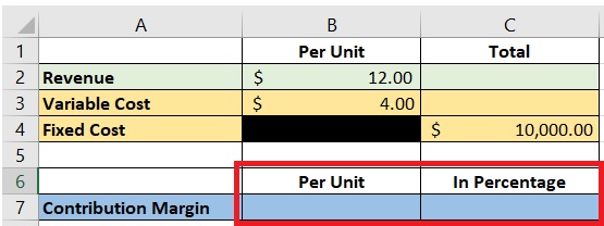
Next, we’ll have to input the formulas for computing the contribution margin.

Contribution margin per unit is simple to compute.

We only need to variable cost per unit from the revenue per unit.

This is how it should appear on your excel sheet:

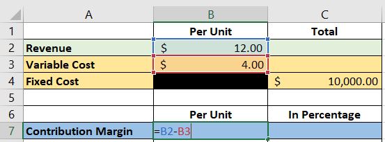
We assigned cell B2 for the revenue per unit, and cell B3 for the variable cost per unit. As such, the formula will be “=B2-B3”.

As for the contribution margin in percentage, we can compute it in two ways:

Contribution Margin = (Total Revenue – Total Variable Costs) ÷ Total Revenue

-or-

Contribution Margin = (Revenue per Unit – Variable Cost per Unit) ÷ Revenue per Unit

We’ll have to put these two formulas in one cell.

To do that, we will be using Excel’s IF function.

The formula using total revenue and total variable costs will be used first.

If we don’t have the data for total revenue and variable cost, we will then use the other formula (which used revenue and variable cost per unit).

This is how it will be presented in excel:

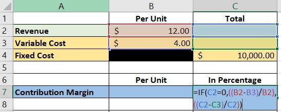
The formula we use is “=if(C2=0,((B2-B3/B2),((C2-C3/C2))”

Using these cells, we can get the contribution margin for our example above:

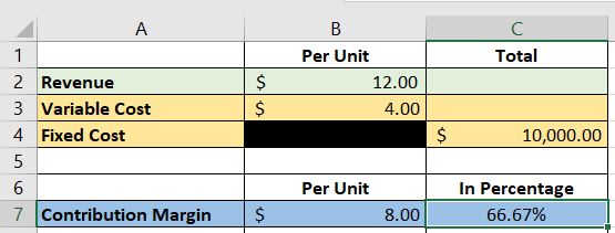
Step 3. Assign cells for the break-even point

And now we’re onto the last step of creating our break-even analysis template.

The break-even point can be expressed in two ways: per unit, or in total revenue.

As such we will be assigning two cells for the break-even point:

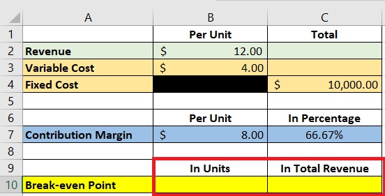
Next, we’ll have to input the formulas for the break-even point.

The formula for the break-even point in units is as follows:

Break-even Point = Fixed Cost ÷ (Revenue per Unit or Variable Cost per Unit)

Or

Break-even Unit = Fixed Cost ÷ Contribution Margin per Unit

We will be using the formula that involves the contribution margin per unit.

This is how it will look like on Excel:

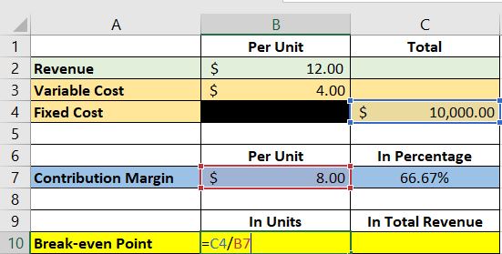
We assigned cell C4 for the total fixed cost, and cell B7 for the contribution margin per unit.

As such, the formula will be “=C4/B7”.

Next, we input the formula for the contribution margin expressed in total revenue.

We use the following formula:

Break-even Point = Fixed Cost ÷ Contribution Margin (in percentage)

This is how it will look like on Excel:

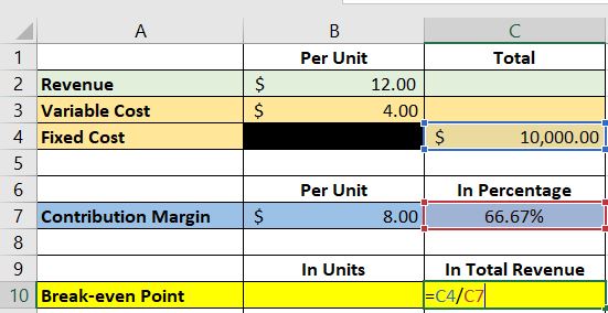
We assigned cell C4 for the total fixed cost, and cell C7 for the contribution margin in percentage.

As such, the formula will be “=C4/C7”.

And with that, we have our break-even analysis template.

Let’s use our newly made template to compute the break-even for our example above:

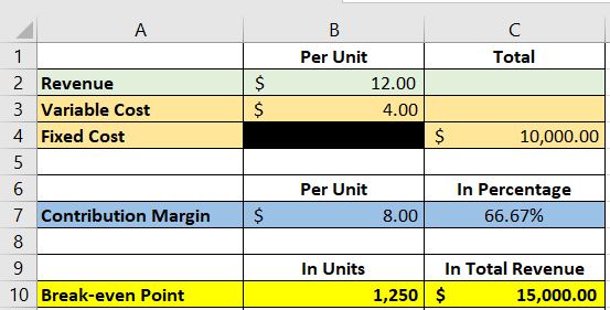
According to our break-even analysis template, we need to sell 1,250 units of the new product or generate a total of $15,000 revenue to fully cover our variable and fixed costs.

If we sell more than these figures, we’ll be able to generate profit.

Extra step. Assign cells for variable and fixed costs at the break-even point

This step isn’t necessary.

But if you want to know what the total variable and fixed costs are at the break-even point, you can continue reading on this section.

If not, you can proceed to the next section.

First, we assign two cells for variable and fixed costs at the break-even point (“per unit”, and “total”):

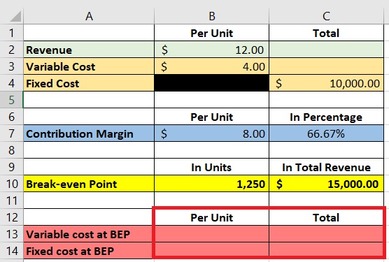
BEP means Break-even Point

We then input the formula for each cell.

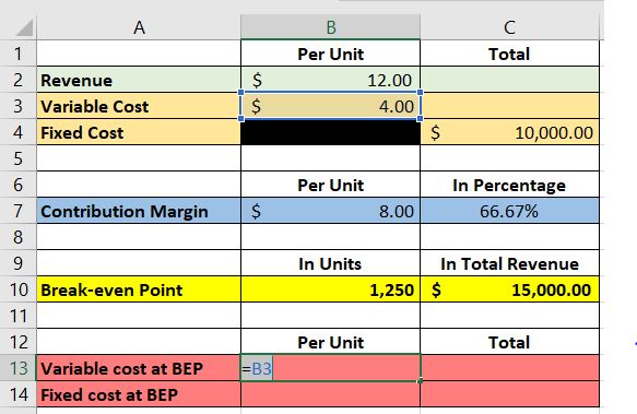
Let’s start with the variable cost per unit.

This is simple as the variable cost per unit would be the same at all levels (when using break-even analysis).

As such, the formula in excel will look like this:

As for the total variable cost at the break-even point, the formula should look like this in Excel:

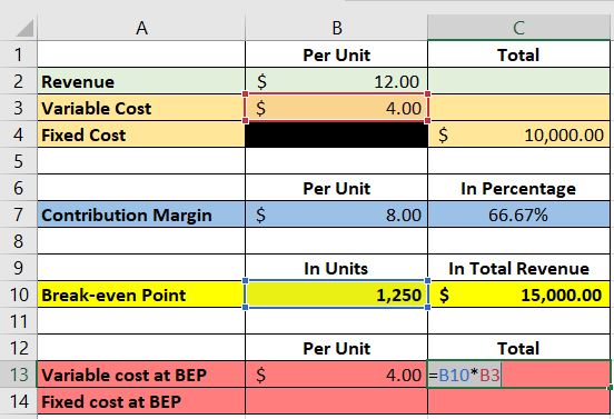
We assigned cell B10 for the break-even point in units, and cell B3 for the variable cost per unit.

You can also use cell B13 instead of cell B3 for the formula.

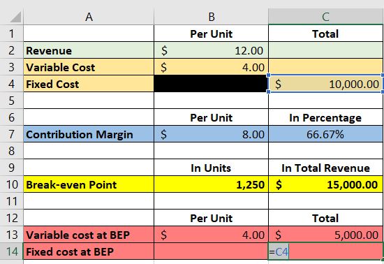
Next, we input the formula for the total fixed cost.

The total fixed cost should stay the same no matter the activity level.

As such, the formula should look like this in Excel:

As for the fixed cost per unit, we will be using the following formula:

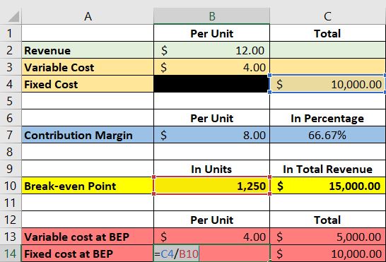
You can use cell C14 instead of C4 for the formula.

Here’s how it should look like after inputting all the formulas:

 

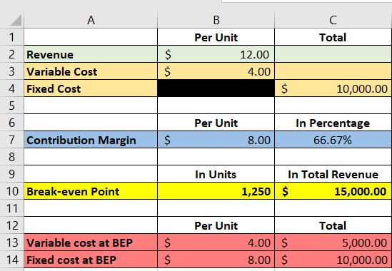
Using Goal-Seek to Perform Break-Even Analysis

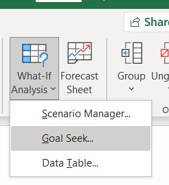
Another way to perform a break-even analysis in Excel is to use the “goal-seek” function.

This is a built-in function in Excel, so you don’t have to download additional plug-ins.

It can be found on the Data tab, under What-If Analysis:

Step 1. Create a template

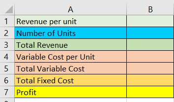
To start, we’ll have to design our template first. For now, let’s make it simple and have at least the following variables:

• Revenue per unit
• Number of Units (sold, produced, etc.)
• Total Revenue
• Variable Cost Per Unit
• Total Variable Cost
• Total Fixed Cost

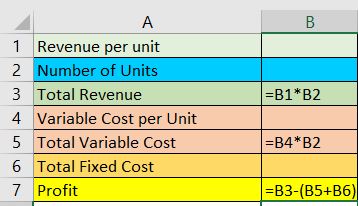
The resulting simple template should look like this:

Step 2. Input formula in cells that need it

Next, we input formulas to cells that need it:

• Total Revenue = Revenue Per Unit x Number of Units
• Total Variable Cost = Variable Cost per Unit x Number of Units
• Profit = Total Revenue – (Total Variable Cost + Total Fixed Cost)

Step 3. Use the Goal-Seek function

Now, we have our completed template.

The next step is to fill in the blanks.

The goal-seek function is useful if you’re missing just one variable (usually the revenue per unit).

For example, let’s say we have the following data regarding a new product that is about to be launched:

• Variable Cost per Unit = $5.00
• Total Fixed Cost = $5,000.00
• Number of Units (expected to be sold) = 800

What we’re missing is the sales price (revenue) per unit.

We want to know the break-even point of this new product.

This is where the goal-seek function comes in.

First, we input all the data that we can on our Excel template:

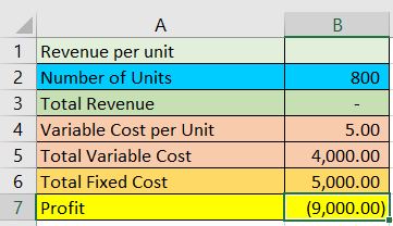
Next, we use the goal-seek function.

The aim is to make the profit zero since there is no profit nor loss at the break-even point:

We assigned cell B7 for the profit figure. We want to change its value to zero.

Next, we want to determine the revenue per unit at the break-even point.

This can be done by completing the Goal-Seek form:

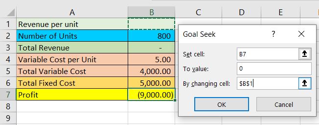
We assigned cell B1 for the revenue per unit figure.

After clicking ok, the values will update, and we should be able to get the revenue per unit at the break-even point:

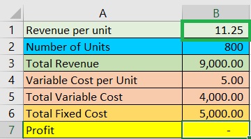
The sales price (revenue) per unit of the product must be $11.25 for it to fully cover its costs.