Extracting Unique Values From Columns in ExcelHere are several methods to remove duplicates in a column
When you work with data in Excel, you’d oftentimes come across datasets that have repeating values (or duplicates) in certain columns.
There is no immediate issue with this happening because some datasets normally function like that.
For example, if you’re working with an Excel file that includes a store’s sales invoice for the month, there probably are duplicates in the column that contains customer names.
Suppose you want to extract the unique values from such columns, what are you to do?
For example, a store is running a contest and it wants a list of all its customer.
But the store wants to exclude duplicates in the list. What are you gonna do to get such a result?
Well as always, you can manually work with the column so that only unique values appear in it.
But that would take time if you’re working with a large size of data. And doing it manually can lead to errors.
Fortunately, there are several efficient ways that you can extract unique values from a column in Excel.
You don’t have to do it manually and risk making a mistake.
It will also save you a lot of time.
So continue reading on to learn these very efficient methods of extracting unique values from a column in Excel.
Why Do You Need to Extract Unique Values From a Column in Excel?
There are several reasons why you want to extract unique values from a column in Excel.
Some of them include the following:
- You suspect that some data are duplicated erroneously. This is easily noticed if there are rows or columns that contain the same data even ones that should be unique. For example, the sales invoice number should be unique for every transaction.
- You want to create a list of data that excludes duplicates. For example, you want to make a list of all customer names. You also want the list to exclude any duplicates so that only unique values are included.
- You want to filter out the Excel sheet so that it only includes unique values.
Using the Remove Duplicates Tool to Extract Unique Values From a Column in Excel
The first method of extracting unique values in Excel is probably the easiest and most popular.
It involves using the Remove Duplicates tool.
What it does is remove any duplicates within your selection. It then returns you with a column that only contains unique values.
How to Use the Remove Duplicates Tool
We will be using the following dataset for illustration purposes:
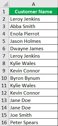
As you look into the data above, you’d notice several names being listed multiple times.
Your goal is to remove duplicates of such names so that you’d come up with a list that only includes unique values.
You’ll do this by using the Remove Duplicates tool.
- Select the range of cells that you want to extract unique values from. In our illustration, that would be cells A2 to A16.
- Open the Data tab. You should find the Data Tools section somewhere in the middle-to-right of the tab. Click on the Remove Duplicates button. This will open the Remove Duplicates window.

- In the Remove Duplicates Window, make sure to check all settings.

- Click the OK button after doing so.

- A message box will pop up informing you how many duplicate values were found within your selection as wiel as how many unique values remain in your list. Click the OK button.

- Your selection should only have unique values now.
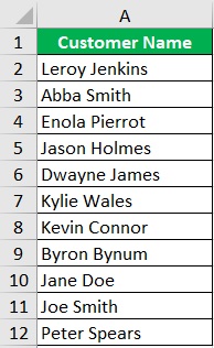
Caveat About The Remove Duplicates Tool
Did you notice that some cells within your selection were deleted?
That’s because the Remove Duplicates tool directly applies any changes to your selection.
That means that it applies the changes to your original data, which isn’t ideal if you want to keep the original list untouched.
So if you want to retain that original data while using the Remove Duplicates tool, it’s recommended that you make a copy of it before you remove duplicates.
Using the Excel Advanced Filter Tool to Extract Unique Values From a Column in Excel
Another method to extract unique values in Excel is to use its Advances Filter tool.
Unlike the Remove Duplicates tool, you have the choice of applying the changes to your selection or displaying the result in a new location.
How to Use the Advanced Filter Tool
We will be using the same dataset for illustration purposes:

Your goal is to remove duplicates from this list using Excel’s Advanced Filter tool.
- Select the range of cells that you want to extract unique values from. In our illustration, that would be cells A1 to A16. Make sure to include the column header in the selection.
- Open the Data tab. You should find the Sort & Filter section somewhere in the middle of the tab. Click on the Advanced button.
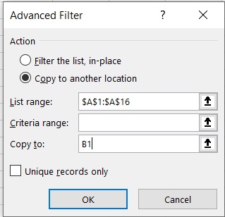
- This will open the Advanced Filter window.

- [Remove duplicates from the original data] If you want to remove duplicates from the original data, tick the button before “Filter the list, in-place”.
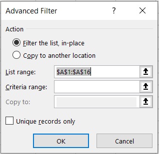
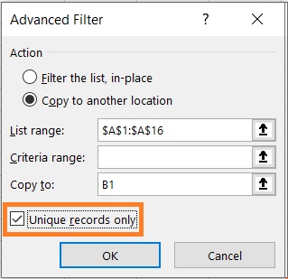
- Tick the box before “Unique record only”. Click the OK button after doing so. This should remove the duplicates from your selection.
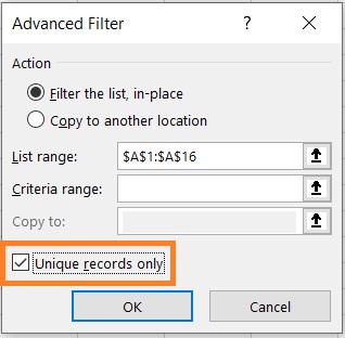
- [Show result in another location] If you want to retain the original data/column and display the unique values in another location, then tick the button before “Copy to another location”. You will also have to fill in the textbox after “Copy to”. This is where the result will be displayed (for our illustration, we want it to be B1 or $B$1).
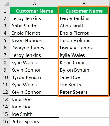
- Tick the box before “Unique record only”. Click the OK button after doing so. This should display the unique values on your “Copy to” location.
Using the UNIQUE Function to Extract Unique Values From a Column in Excel
One of the newest functions that have been added to Excel 365 is the UNIQUE function. Similar to the previous tools, the UNIQUE function returns a list of unique values from your selection. However, it also has additional options such as only including values that don’t have duplicates or extracting unique values from multiple columns.
The formula for using the UNIQUE function is as follows:
=UNIQUE(array, , )
Where:
array – refers to the range of cells from which you’ll be extracting unique values
[by_col] – specifies whether the UNIQUE function extracts unique values by rows or columns. This is a TRUE/FALSE or 0/1 value and is FALSE by default (which means that it extracts unique values by rows by default.
[exactly_once] – specifies whether or not you want to extract only values that appear once within the selection. By default, its value is FALSE which prompts the function to return a list of values that appear at least once within the selection. If the value is TRUE, the function will instead return a list that only has values that only appear once within the list.
The last two parameters are optional. If you only want to extract unique values from your selection, then you can simply use the formula =UNIQUE(array).
How to Use the UNIQUE Function
We will be using the same dataset for illustration purposes:

Your goal is to remove duplicates from this list using the new UNIQUE function.
- Select a cell where you want present the list of unique values. This cell as well as the column where it belongs should be empty for the function to work properly. For our illustration, this cell will be cell B2.
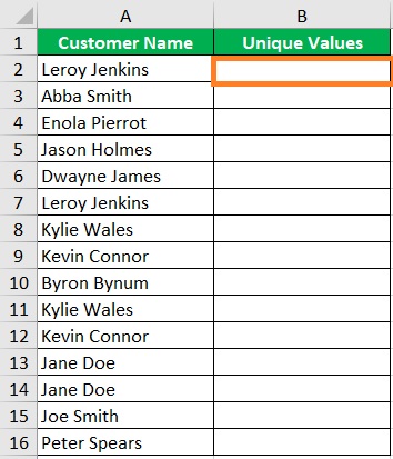
- Type the formula for the UNIQUE function in the selected cell. For our illustration, the formula will be =UNIQUE(A2:16). This will create a list of unique values from cells A2 to 16 in column B starting from cell B2.

- Press the ENTER key. The UNIQUE should return a list of unique values from your selection.

Do note that this function is dynamic. It will automatically update the list if there are changes in the selection.
Combining the IF and COUNTIF Functions to Extract Unique Values From a Column in Excel
Combining the IF and COUNTIF functions is an interesting way to extract unique values in Excel. It isn’t as intuitive as the previous methods. But if you’re already familiar with these formulae, you might want to give this method a try. Unlike the other methods, the list will have blank cells. However, it will automatically update if there are any changes in the selection.
Let’s say that the selection from which we want to extract unique values start in cell A2. The formula will look like this:
=IF(COUNTIF(A$2:A2,A2)=1,A2,””)
Combining the IF and COUNTIF Functions
We will be using the same dataset for illustration purposes:

Your goal is to make a list of unique values by combining the IF and COUNTIF functions.
- Select a cell where you want present the list of unique values. This cell as well as the column where it belongs should be empty. For our illustration, this cell will be cell B2

- In your selected cell, type the formula that combines the IF and COUNTIF function. For our illustration, the formula will be =IF(COUNTIF(A$2:A2,A2)=1,A2,””).

- Press the ENTER key. Then copy the formula and paste it into the rest of the cells in the same column up until the next empty row.

- You should now have a list of unique values. You’ll notice that there are blank cells. That is the IF function at work. If the COUNTIF function counts more than 1 of the value within its selection, the IF function will return a blank.

Conclusion
And there you have it.
Several ways of extracting unique values from a column in Excel.
I hope you are able to find a method that suits your preference.
