How To Split Single Column into Multiple Columns in Microsoft ExcelStep by Step Guide


In Microsoft Excel, the way you construct and arrange your data is important.
It is easy to understand and read data when the information is arranged well and presented clearly.
To make the tables readable, you will need to organize your data into groups.
That way, managing the information is easier.
If you are the one who created the project in Excel from scratch, you know how the data was constructed and ensured the information is readable.
The real challenge is if the project you are working on is created by someone else, especially if there is a lot of data.
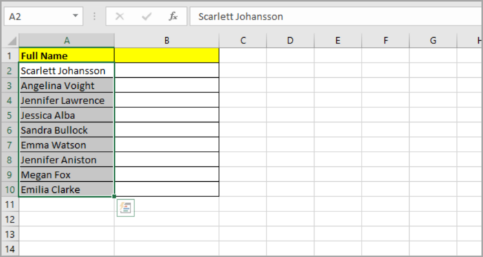
For example, arranging lists like names takes a lot of effort to finish, and sometimes you are required to arrange it alphabetically.
See the table below:

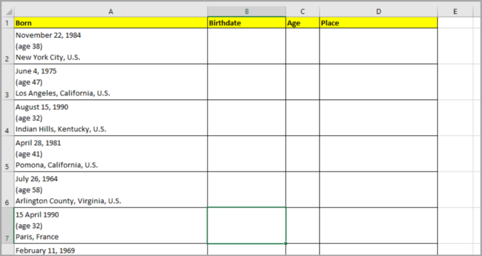
You may also be given lists of birth details and additional related information, and you want to arrange it properly to make the information easier to read.
The best way to organize the two problems above is to split one column into multiple columns depending on how much data you are working on.
Newer versions of Microsoft Excel give a feature that lets you do that by using the ‘Data’ menu.
Let’s now see how you can use this feature.
Splitting a Single Column into Multiple Columns
Let’s say that you are given the list of names and you are required to split the name and surname into different columns.
- Click/select the column that you chose to split.

- Go to the Data Menu, then click the “Text to Columns” located in the Data Tool group. The Convert Text to Column Wizard will appear.

- In this option that appears, you will see the Delimited and Fixed widths. Now make sure that you select Delimited. Delimited is the character that states how the data that you selected in the cell separates from one another. For example, the image above gives us the name and surname of that specific person in one cell separated by a space between them. Now the space that is in between the name and surname is our delimiter.

- Click the Next button.
- Settings you need to do/check in the second step of the Text Column Wizard:
- The ‘Tab’ delimiter is the default checked. But in this instance, we are not using Tab. Instead, we are using the ‘Space’ delimiter. So, uncheck the ‘Tab’ and check Space’.
- You also need to check ‘Treat consecutive delimiter as one’. This checkbox means that if you accidentally put two spaces between the names, you will treat the space as only one.
- In the bottom area, you will now see the preview area of the result of your data.
- Lastly, click the Next Button.

- You will see an option where you can state the format for your data in the column. You will see in the option the General option is ticked. This means that you are using the same format as the original cell. In this case, just leave the General ticked, then press the Finish button.

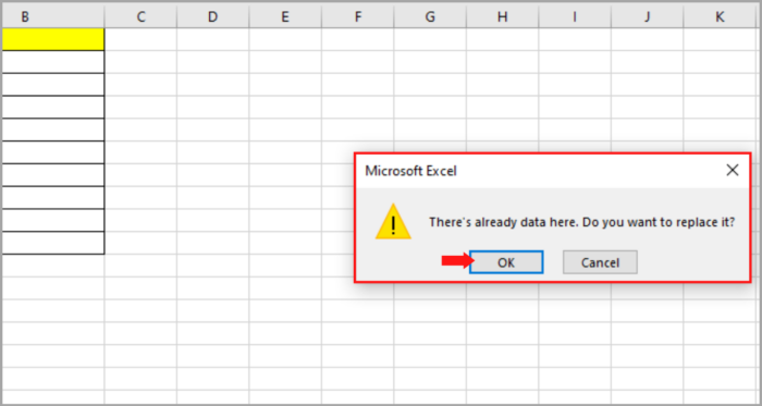
- Sometimes there is a message in the dialog box that asks if you want to “replace the data” that is already present in the destination cells. Just Click OK.
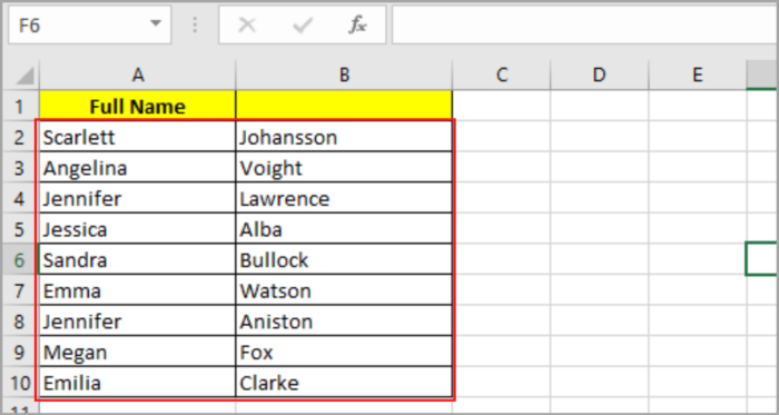
From one single cell, we have now separated it into two cells. Column A is for the name and column B is for the surname.
Take note that when you split the names in the cell, Excel should not insert new cells to hold the names.
You should leave an empty cell on the right before you begin to split the cell.
This is because the new cell will overwrite the existing cells. You will also have the choice to select where you want to locate the split data.
When it comes to the number of columns, this will depend on how many delimiters you have selected.
If you have given three words to split you can use a comma as your delimiter to separate the given single column into multiple columns.
Splitting Multiple Lines in a Cell into Multiple Cells
Sometimes you are given multiple lines into a single cell. In this scenario, we will separate the multiple lines into multiple cells.
See our given data below:

As you can see, we are given multiple pieces of information, namely, their names, Streets, Cities, and Countries. We are going to separate these given data into multiple cells.
Unfortunately, it is not that simple to split the above information. It’s not impossible either. Here is the step-by-step process of how to do it:
- Click and select the column you chose to split.
- Go to ‘Data” and select ‘Text to Columns’. The Convert Text to Column Wizard will appear.
- Now choose the delimited option.
- Then, click the Next button.
- From here you will see the ‘Tab’ option checked. Uncheck all of it and check the ‘Other’ option. Then choose the delimiter character you want to use. We will use the CRTL key + J shortcut on your keyboard because we want to use line-break characters. There will be a tiny blinking dot inside the box. The delimiter you chose is now inserted.
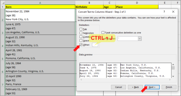
You can now see the result in the data preview area located at the bottom part of the dialog box.
This is the result we wanted. The separation of information is now located in different cells. The first column is for the names, the second column is for the Street, the third column is for the City and lastly the fourth is for the country.
- Click the Next button.
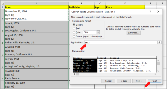
- You will see an option where you can state the format for your data in the column. You will see in the option the General option is ticked. This means that you are using the same format as the original cell. In this case, just leave the General ticked, then press the Finish button.
- We want all the columns to appear in column B onwards. Because In this case, we don’t want to overwrite the information in the first cell. In the Destination, type ‘$B$2’, this means we will start at column B2. Then click the Finish button.
- Sometimes there is a message in the dialog box asking if you want to “replace the data” that is already present in the destination cells. Just Click OK.

Now you are done. You can see in the picture below that the information in the first column is separated into different columns.

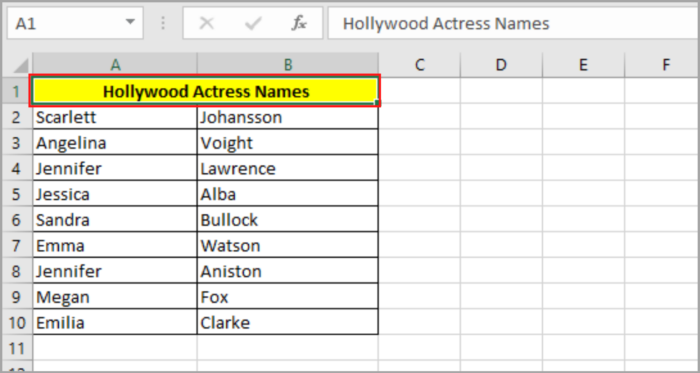
Splitting up a Merged Cell
Another feature of Excel is spitting up a merged cell. If you are given a merged cell and you want to split or unmerge the cell, here are the steps on how you can unmerge the cells:
- Select all the merged cells. If you are given a lot of data and you need to unmerge them, simply select all of them.
- Go to the Home Tab. In the alignment tools, you will see the Merge & Center option. Click it, a drop-down menu will appear, and select “Unmerge Cell”.
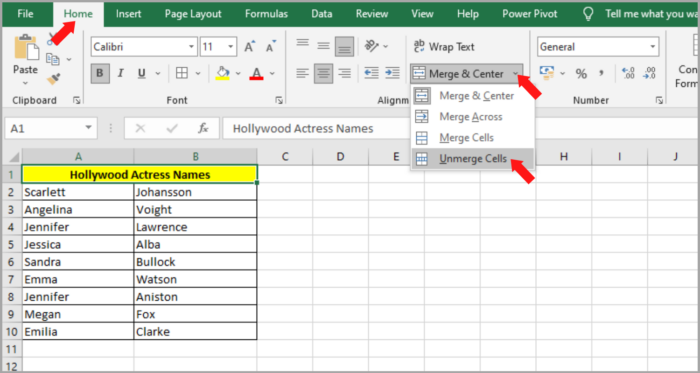
- This will now split your merged cell back to its original quantity of cells.
You cannot split into smaller cells any cell that is not merged, unlike in MS Word.
Conclusion
In this tutorial, we discussed how we can split data from a single cell into multiple cells in Excel by using different types of delimiters and how it actually works.
In addition, we also looked at examples of how we can split cells that have been recently merged.
The steps that we tackled are best to use in the newer versions of Microsoft Excel, specifically versions 2013 to 2019.
Microsoft automatically updates its software so you can enjoy the latest features that are available.
Note that not all versions of Excel may run these steps, especially the older versions.
I hope this helps you a lot!