20 Must-Know Advanced Excel Functions (with Formulas)Up your Excel game with these advanced functions

Last Updated: March 8, 2023

Written By:
Patrick Louie

Excel has tons of functions, all of which have roles to play.

These functions can be typically accessed via a formula.

Some of them are simple such as the SUM and COUNT functions. Some of them are advanced (ones that require minimum know-how about the function).

Then there are those that work best when paired with each other (such as the INDEX-MATCH combo).

As of Excel 2016, there are 484 functions that an Excel user can access via formulas and VBA codes.

That’s a lot, isn’t it? Well, while each function has its proper use, it’s not like you’ll be using them all.

Most likely, you’ll only be frequently using some of them.

While some of them, you only use occasionally (or maybe not at all).

Maybe you already know how the simple functions (or most of them) work and are wanting to expand your repertoire of Excel functions.

Or maybe you’re an advanced Excel user who just needs a quick list of the must-know advanced Excel functions.

Whichever the case, I’m sure that you’ll be wanting this article.

That’s because, in this article, we will be talking about 20 advanced Excel functions that anyone must know to unlock Excel’s full potential.

Hint: VLOOKUP, one of Excel’s most popular functions, is one of them.

Let’s get started!

#1: VLOOKUP

The VLOOKUP is of the most popular Excel functions (probably the most popular even).

Some consider it a rite of passage. If you know VLOOKUP, you know Excel… well that may be an exaggeration.

But, the utility the VLOOKUP provides isn’t an exaggeration. There’s a reason why VLOOKUP is popular.

It is one of Excel’s lookup and reference functions. What it does is look up an array for a key value (the lookup value).

It then returns a value from a different column (which you specify) that matches the row of the key value. Here’s an illustration of VLOOKUP in action:

[1] this is the key value (a.k.a. lookup value)

[2] this is the lookup array

[3] these are the VLOOKUP formula and the result

The formula to use VLOOKUP is as follows:

=VLOOKUP(lookup_value,array,col_index_num,[range_lookup]

#2: INDEX-MATCH Combo

The INDEX-MATCH combo works like a lookup and reference function.

This combination of functions is even more versatile than the more popular VLOOKUP.

What holds it back from being more popular than VLOOKUP is its relatively more complex formula.

That, and the fact that it’s a combination of two functions that don’t do much on their own.

INDEX-MATCH can do all the things VLOOKUP can and more:

It doesn’t have the limitations of requiring the results column/value to be to the right of the lookup value
It can both function horizontally and vertically
Unlike VLOOKUP’s static column reference, the INDEX-MATCH combo makes a dynamic reference to the results column

Personally, I prefer the INDEX-MATCH combo over VLOOKUP, but I can understand why the latter is more popular.

The formula for using the INDEX-MATCH combo is as follows:

=INDEX(array,MATCH(lookup_value,lookup_array,[match_type]))

(Here’s an article that demonstrates how the INDEX-MATCH combo works: Perform Reverse VLOOKUP in Excel)

#3: XLOOKUP

XLOOKUP is another lookup and reference function.

It’s probably the most powerful and most useful among all the lookup and match functions at the very least.

Having said that, many will still use VLOOKUP over the objectively superior XLOOKUP.

Why is that? It’s because the XLOOKUP is only available in Excel 2021 and Excel 365.

Its limited availability is what’s holding it back from becoming the most popular Excel function.

But given the time when it becomes more available, I am confident that it will be more widely used than VLOOKUP or INDEX-MATCH.

XLOOKUP virtually does the same things as the INDEX-MATCH combo.

It can perform vertical and horizontal lookups, and it doesn’t have the limitations that VLOOKUP has.

Its edge over the INDEX-MATCH combo is that it’s a stand-alone function. Thus, it has a relatively simpler formula:

=XLOOKUP(lookup_value, lookup_array, return_array, [if_not_found], [match_mode], [search_mode])

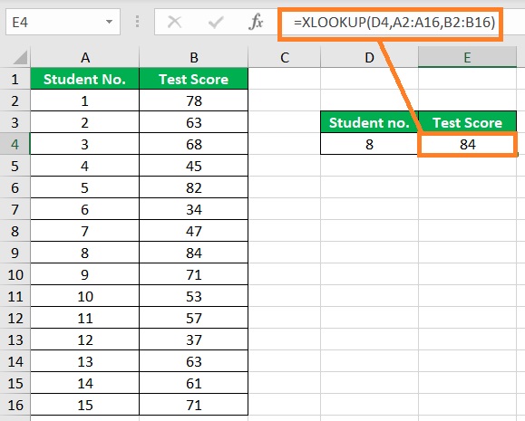
It requires 6 arguments, but only 3 of them are mandatory. The other 3 are optional. Here it is in action:

As you can see from the formula above, I only made the 3 mandatory arguments for XLOOKUP to work properly.

#4: IFS

The IF function lets you set up at most two conditions on its own.

You can still add more conditions by nesting multiple functions though.

However, that often leads to a long nested IF formula.

Just imagine having to check for 10 or 20 conditions by nesting multiple IF formulas. Not a pretty sight, I tell you.

Thankfully, there’s the IFS function that can do away with all the nesting of multiple IF formulas.

With the IFS function, you can set as many conditions as you want. It was introduced in Excel 2019.

The formula to use the IFS functions is as follows:

=IFS(logical_test1,value_if_true1, logical_test2,value_if_true2…)

Here’s a comparison of the IF and IFS functions with the same conditions:3

#5: SUMIF/SUMIFS

The SUMIF and SUMIFS functions perform similar actions: they add the values that meet the stated condition/s from a selected range of cells.

Where they differ is the number of conditions that you can set. For SUMIF, you can only set one condition (a.k.a. logical test). For SUMIFS, you can set multiple conditions. Use the appropriate function according to your need.

For example, if you want to know the total sales amount made by a particular sales agent, then it’s better to use the SUMIF function as you only need to set one condition.

If you want to know the aggregate sales amount by two or more particular sales agents, it’s better to use the SUMIFS function.

The formula for the SUMIF function is as follows:

=SUMIF(range,criteria,[sum_range])

The formula for the SUMIFS function is as follows:

=SUMIFS(sum_range,criteria_range1,criteria1,criteria_range2,criteria2,…)

#6: COUNTIF/COUNTIFS

The COUNTIF and COUNTIFS functions are like the SUMIF and SUMIFS functions but instead of adding the values, they count the values.

For example, the COUNTIF function can count the number of products made by a particular worker.

The COUNTIFS function can count the aggregate number of products made by two workers or more.

The formula for the COUNTIF function is as follows:

=COUNTIF(range,criteria)

The formula for the COUNTIFS function is as follows:

=COUNTIFS(criteria_range1,criteria1,criteria_range2,criteria2,…)

#7: IFERROR

Even if you already are an expert in Excel, you may still come across error values such as #N/A or #DIV/0! from time to time.

These error values are often a result of faulty formula arguments. But sometimes, they may be out of your control.

The IFERROR function allows you to substitute these error values with a more meaningful description such as “Cannot divide by zero” or “Data not found”.

This communicates the error much better to other users of the sheet.

The formula for using IFERROR is as follows:

=IFERROR(value,value_if_error)

#8: SUMPRODUCT

At first glance, you may find SUMPRODUCT as a simple function that works similarly to the SUM function.

Well, I wouldn’t blame you. It was originally intended to calculate the of the product in two columns.

But, it can be more than that. Eager Excel users were able to find another use for SUMPRODUCT: it can be used for conditional sums or conditional calculations.

By that, I say that it can function the same as the SUMIFS function.

For example, it can add up values that are greater than a specific value.

The formula for using SUMPRODUCT is as follows:

=SUMPRODUCT(array1,array2,array3…)

#9: OFFSET

The OFFSET function does a simple task, but for you to use it effectively, you need to understand how it works.

It returns the value in a cell that is n columns and n rows away from the reference cell.

For example, I can use OFFSET to retrieve the value that is 2 rows below and 2 columns to the right of cell A2 (which is the value in cell C4).

The formula to use OFFSET is as follows:

=OFFSET(reference,rows,cols,[height],[width])

Where

reference – this refers to the reference cell

rows – this defines how many rows away the value is from the reference. It can go up or down. Setting it as a positive number means that the value is n rows below the reference. Setting it as a negative number means that the value is n rows above the reference

cols – this defines how many columns away the value is from the reference. It can go to the left or the right. Setting it as a positive number means that the value is n columns to the right of the reference. Setting it as a negative number means that the value is n columns to the left of the reference

[height] and [weight] – these specify the height and weight that you want the returned reference to be

#10: TEXTJOIN

The TEXTJOIN function is essentially an upgrade of the CONCATENATE function.

With it, you can quickly combine the contents in a selected range of cells. The best part about is that you don’t have to use the & symbol a lot of times.

Another feature that it has that CONCATENATE doesn’t is allowing you to specify a delimiter that will delimit that content between the combined cells.

The formula for using TEXTJOIN is as follows:

=TEXTJOIN(delimiter,ignore_empty,text1,text2,text3…)

If you’re using the latest version of Excel (or Excel 365), you should be using the TEXTJOIN function instead of CONCATENATE.

#11: FILTER

The FILTER function is the first array function that we’ll be talking about in the article (but it certainly won’t be the last).

It’s not to be confused with the always-there filter feature of Excel, though it does the same thing.

The FILTER function returns an array that contains only the values that meet the condition set in the formula.

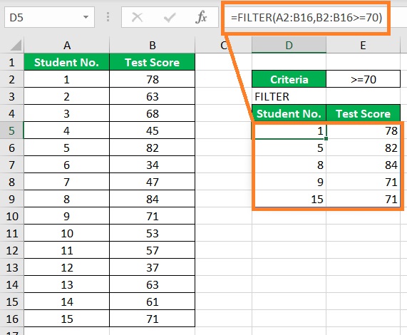
For example, I want to retrieve the student numbers and test scores of students who earned at least a 70 test score.

Here’s how I would do it with the FILTER function:

Since it is an array function, it will return an array that is similar in shape to the reference array (in this case, the same number of columns).

The formula to use FILTER is as follows:

=FILTER(array,include,[if_empty])

#12: SORT and SORTBY

The SORT and SORTBY function are another set of array functions.

They’re not to be confused with the always-there sort feature of Excel.

Unlike the sort feature which always gives a static result the SORT and SORTBY give a dynamic array that automatically updates if there are any changes to the referenced array.

With the SORT function, you can quickly sort a range of cells. You can base it on a row or column.

You can also choose the sort order (ascending or descending). It will return an array with values of the reference sorted according to the sorting order that chose.

On the other hand, the SORTBY function allows you to sort a range of cells or an array based on multiple columns.

The formula for using SORT is as follows:

=SORT(array,[sort_index],[sort_order],[by_col])

The formula for using SORTBY is as follows:

=SORTBY(array,by_array1,[sort_order1],[by_array2,sort_order2],…)

#13: UNIQUE

UNIQUE is another array function. This function returns a dynamic array that contains only the unique or distinct values from a dataset or an array. That’s it.

It made the act of retrieving unique or distinct values quicker and easier.

Before, you’d have to use the remove duplicates feature of Excel just to get the distinct values.

And for unique values, you have to use a combination of functions. But with UNIQUE, you only need one function.

The formula for using UNIQUE is as follows:

=UNIQUE(array,[by_col],[exactly_once])

The optional argument [exactly_once] lets you set whether you want to retrieve unique or distinct values.

#14: SEQUENCE

SEQUENCE creates an array but it does not base its result on another array (reference array).

You can use it on an empty sheet and it will still work out fine. As the name suggests, SEQUENCE gives you an array that contains a sequence of numbers.

You can specify how many rows and columns the resulting array will have. You can also specify the starting number as well as how far the next number will be.

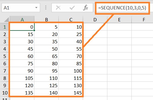
For example, I can make an array of sequential numbers with 10 rows and 3 columns.

The sequence will start at 0 and the numbers are 5 digits apart. Here’s what it would look like:

The formula for using SEQUENCE is as follows:

=SEQUENCE(rows,[columns],[start],[step])

#15: SMALL and LARGE

SMALL and LARGE are two pretty simple functions.

SMALL returns the nth smallest value from the referenced range of cells. On the other hand, LARGE returns the nth largest value from the referenced range of cells.

On their own, they are pretty simple functions.

Where they became advanced is when you use them in combination with other functions.

For example, you can use either of the two with VLOOKUP or XLOOKUP.

The formula for using SMALL is as follows:

=SMALL(array,n)

The formula for using LARGE is as follows:

=LARGE(array,n)

#16: RIGHT, LEFT, and MID

RIGHT, LEFT, and MID are text-related functions.

You can use any of them to extract a part of a text string.

RIGHT lets you extract from the right, while LEFT lets you extract from the left. MID lets you extract text from the middle of the text string.

On their own, they’re pretty simple functions.

All they do is return a portion of a text string.

However, they are often used in advanced formulas (with the LEN or FIND functions).

The formula for using RIGHT is as follows:

=RIGHT(text,[num_chars])

The formula for using LEFT is as follows:

=LEFT(text,[num_chars])

The formula for using RIGHT is as follows:

=MID(text,start_num,num_chars)

#17: FIND and SEARCH

FIND and SEARCH are two functions that work similarly.

They both allow you to search for a particular text in a cell. Both then return the starting position of the text that you searched for.

They aren’t that much use on their own. But with other functions text functions such as RIGHT, LEFT, and MID, you can perform various levels of text manipulation.

The formula for using FIND is as follows:

=FIND(find_text,within_text,[start_num])

The formula for using FIND is as follows:

=SEARCH(find_text,within_text,[start_num])

Do not that you can’t use wildcard characters with FIND. They’re fine with SEARCH though.

#18: REPLACE and SUBSTITUTE

REPLACE and SUBSTITUTE are two functions that work similarly.

They allow you to find a particular text in a text string, then replace or substitute it with a new text value. How they do the task is a bit different.

With REPLACE, you’ll have to specify the starting position of the text as well as the number of characters that you want to replace within the text string.

Meanwhile, with SUBSTITUTE, you’ll have to specify the text that you want to substitute with the new value.

SUBSTITUTE works best if you know the text that you want to replace. On the other hand, REPLACE works best if you consistently want to replace the characters in the nth place of the text string.

The formula for using REPLACE is as follows:

=REPLACE(old_text,start_num,num_chars,new_text)

The formula for using REPLACE is as follows:

=SUBSTITUTE(text,old_text,new_text,[instance_num])

#19: TEXTAFTER and TEXTBEFORE

TEXTAFTER and TEXTBEFORE are another set of text functions. They work similarly to the LEFT/FIND and RIGHT/FIND combinations. Currently, they’re only available in Excel 365. With TEXTBEFORE, you can extract all the text before a specified delimiter. On the other hand, you can extract all the text after a specified delimiter with TEXTAFTER.

The formula for using TEXTAFTER is as follows:

=TEXTAFTER(text,delimiter,[instance_num],[match_mode],[match_end],[if_not_found])

The formula for using TEXTBEFORE is as follows:

=TEXTBEFORE(text,delimiter,[instance_num],[match_mode],[match_end],[if_not_found])

#20: WORKDAY and NETWORKDAYS

WORKDAY calculates the date after a particular number of working days (from a reference date).

On the other hand, NETWORKDAYS calculates the number of working days between two dates. Pretty simple to understand, right?

The fun doesn’t end there though. You can customize how these functions work.

You can specify which holidays to ignore in the calculation.

Also, you can specify what are the work days.

Some workplaces have a mon-fri workweek while some have a mon-sat. They also work for part-time arrangements.

The formula for using WORKDAY is as follows:

=WORKDAYS(start_date,days,[holidays])

The formula for using NETWORKDAYS is as follows:

=NETWORKDAYS(start_date,end_date,[holidays])

Conclusion

And those are the 20 must-know advanced functions in Excel.

Having these functions in your arsenal will help you in unlocking the full potential of Excel.

Did I miss an important Excel function?

Let me know in the comments.