Perform Reverse VLOOKUP in ExcelLearn how to perform reverse VLOOKUP with these function combinations


Excel has tons of functions and features that make working with a large dataset easier and more efficient.
For example, there are functions or function combinations that can help you retrieve a certain value from a table or array based on a key value or criterion.
One such function is VLOOKUP (short for Vertical Lookup).
With VLOOKUP, you can search for a certain value in a column to retrieve a value from a different column in the same row.
Here’s an example:

What VLOOKUP example above is to search for the key value (which is in cell F3) in the table array (which is the range of cells A2:C32).
Then it returns a value from a different column in the same row. In the illustration above, the column of the returned value is specified to be the 2nd column of the table array.
Now while VLOOKUP is a very useful function, it has one major limitation.
For it to work, the key value must be located at the most left column of the table array.
This means that VLOOKUP can only look up values to the right. If you work with several datasets, you’ll know that not all of them are structured to address that limitation.
If you try to do so, this is the result:

The VLOOKUP function returned an error value.
This is because the key value is located in the rightmost column of the table array.
Thus, the function will not work properly because there are no values to lookup into to the right. The returned value that we’re looking for is to the left of the key value.
To address this limitation, we have to improvise.
We have to perform a reverse VLOOKUP. Here are ways you can do so.
Use XLOOKUP to Perform a Reverse VLOOKUP
For the first method, we’ll be using the XLOOKUP function. It is one of Excel’s lookup functions (the other being HLOOKUP and VLOOKUP).
It actually acts as a replacement for the other two functions as it does not have the limitations of both.
Unlike VLOOKUP which can only look for values to the right, XLOOKUP can look for values to both the left and right. Thus, we can use it to perform a reverse VLOOKUP.
XLOOKUP is currently available in the most recent versions of Excel (Office 365, Excel 2021).
The formula for using XLOOKUP to perform a Reverse VLOOKUP is as follows:
=XLOOKUP(key_value,lookup_array,results_array)
Where
key_value – refers to the key value or criterion which the function will base on for its search
lookup_array – refers to the array from which the function will look for the key_value
results_array – refers to the array from which the function retrieves the value that matches the row of the key_value
To understand the formula better, let’s have an example:
How to Perform a Reverse VLOOKUP
For illustration, we’ll be using the following dataset:
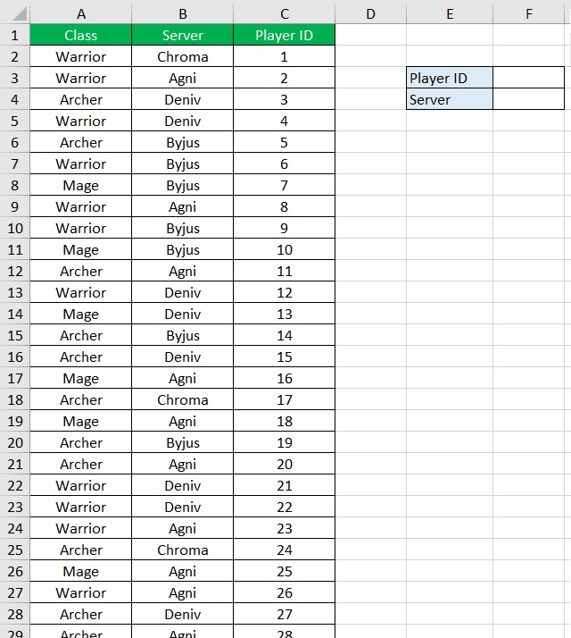
This is a list of player IDs with their corresponding Servers and Classes. It actually has 300 entries.
We’ll be using XLOOKUP to see which server a particular player belongs to (via Player ID). Let’s say we’re looking for which server player 113 belongs to.
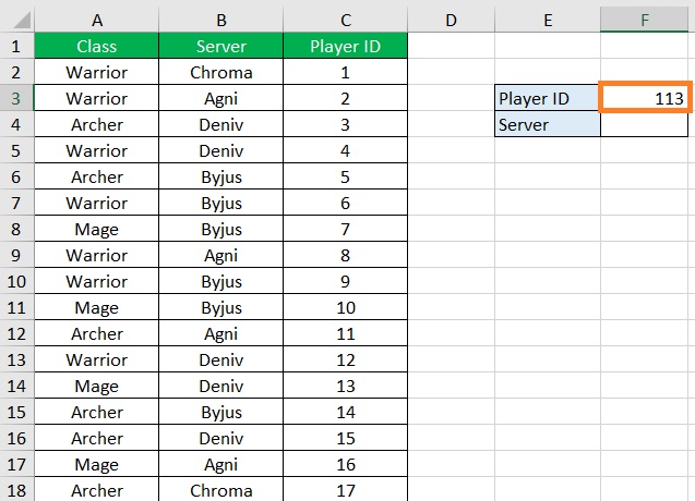
- In cell F3, enter 113.
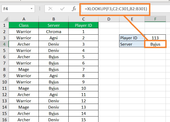
- In cell F4, enter the XLOOKUP formula. For our illustration, the formula will be =XLOOKUP(F3,C2:C301,B2:B301). We set key_value to F3 because it is the cell that contains the criterion for the search. Then, we set lookup_array to C2:C301 because this is the range of cells that contains the Player ID values. Lastly, we set results_array to B2:B301 because this is the range of cells that contains the value that we want the function to return (which is the Server value).

- Press the Enter key. The XLOOKUP function should now return the Server value that corresponds to our specified Player ID value.
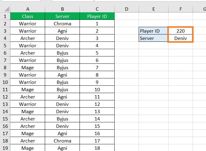
- We have successfully performed a reverse VLOOKUP. If we want to look at which server another player belongs to, we only need to change the Player ID value in cell F3. For example, let’s see which server player 220 belongs to.
Remember that XLOOKUP is only available in the 2021 and Office 365 versions of Excel. If you’re using a version that is not one of these two, you’ll have to use a different method to perform a reverse lookup.
Combine the INDEX and MATCH Functions to Perform a Reverse VLOOKUP
For the next method, we’ll be using a combination of the INDEX and MATCH functions.
The INDEX function returns a value according to the parameters that you set (which are the reference/array, row_num, and column_num(optional)).
On the other hand, the MATCH function searches for a specified value in an array or range of cells and then returns its relative position in the range.
Thus, if we set the row_num of the INDEX formula to the MATCH formula, we’ll get the value from the INDEX reference (or results_array) that matches the row of the specified value.
The formula for this combination is as follows:
=INDEX(results_array,MATCH(key_value,lookup_array,0))
Where
key_value – refers to the key value or criterion which the function combination will base on for its search
lookup_array – refers to the array from which the function combination will look for the key_value
results_array – refers to the array from which the function combination retrieves the value that matches the row of the key_value
How to Perform a Reverse VLOOKUP
For illustration, we’ll be using the following dataset:
This is a list of player IDs with their corresponding Servers and Classes. It actually has 300 entries.
We’ll be using a combination of the INDEX and MATCH functions to see which server a particular player belongs to (via Player ID).
Let’s say we’re looking for which server player 113 belongs to.
- In cell F3, enter 113.
- In cell F4, enter the formula for the combination of the INDEX and MATCH functions. For our illustration, the formula will be =INDEX(B2:B301,MATCH(F3,C2:C301,0)). We set key_value to F3 because it is the cell that contains the criterion for the search. Then, we set lookup_array to C2:C301 because this is the range of cells that contains the Player ID values. Lastly, we set results_array to B2:B301 because this is the range of cells that contains the value that we want the function to return (which is the Server value).

- Press the Enter key. The XLOOKUP function should now return the Server value that corresponds to our specified Player ID value.

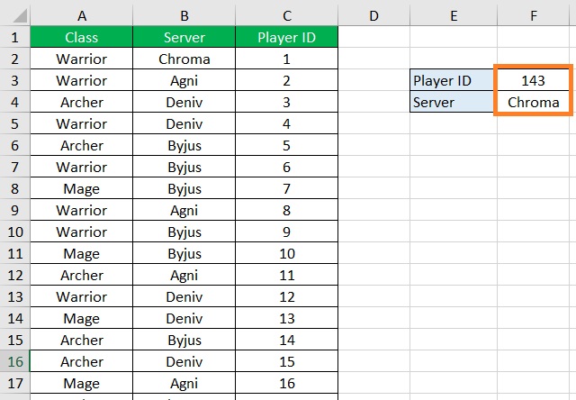
- We have successfully performed a reverse VLOOKUP. If we want to look at which server another player belongs to, we only need to change the Player ID value in cell F3. For example, let’s see which server player 143 belongs to.
Combine VLOOKUP and CHOOSE to Perform a Reverse VLOOKUP
For the last method, we’ll be combining the VLOOKUP and CHOOSE functions.
We already know what VLOOKUP does, but what does the CHOOSE function do?
Basically, it returns a value from a list or array that is based on a specific position.
But we can also use the CHOOSE function to rearrange the columns of a table (without actually rearranging the columns themselves).
It’ll be easier to understand with an example.
Let’s use the same dataset.
Let’s take a look at which server player 143 belongs to by using a combination of the VLOOKUP and CHOOSE functions.
How to Perform a Reverse VLOOKUP
- In cell F3, enter 143.

- Here, the column that the specified belongs to is the rightmost column of the table. This means that VLOOKUP will not work properly unless we rearrange the columns. To do so, we will substitute the table_array to the CHOOSE function. The formula will then be: =VLOOKUP(F3,CHOOSE({3,2,1},A2:A301,B2:B301,C2:C301),2,0). What the CHOOSE function did here is set the order of the arrays we specified and arrange them to the set index order. So A2:A301 becomes the third column, B2:B301 becomes the second column, and C2:C301 (the array that contains the specified value) becomes the first column. Thus, VLOOKUP can now function properly because the column that contains the specified value is now the leftmost column.

- Press the Enter. The formula should now return the Server value that matches the Player ID value. With that, we have successfully performed a reverse VLOOKUP.

Conclusion
To address the limitation of VLOOKUP, we have to get creative.
I’ve just shown you the different ways to perform a reverse VLOOKUP.
I hope that you’re able to use your learnings here in your future endeavors.