High-Low Method in AccountingWhat is it and how to use it for your business

Running a business comes with operating costs.

If you’re employing people, you have to pay their salaries and wages.

If you’re renting a building or space for your business operations, you have to pay rent.

Even if you own the building that houses your operations, you’d still incur costs in the form of depreciation.

Revenue generation often comes with a cost, or rather, costs.

The costs that come with the manufacturing or sale of a product or service can be categorized into three types: variable costs, fixed costs, and mixed costs.

Variable costs are costs that increase or decrease along with the level of activity.

Fixed costs, on the other hand, are costs that remain the same no matter how much is sold or produced (within a certain level of activity).

Mixed costs, as the name implies, are costs that are a mix of variable and fixed costs.

It’s important to know and understand which costs belong to which category.

As you might expect, the cost of sales or manufacturing typically goes up the higher the level of activity is.

It’d be bad if you were planning to manufacture a certain amount of products, yet couldn’t fully understand the costs that come with it.

So if you’re preparing a budget for your business, having an understanding of which cost is which will go a long way.

Thankfully, there are many tools available that can help you in identifying and managing variable, fixed, and mixed costs.

One of these tools is the so-called high-low method. In this article, we will be learning what the high-low method is and how it can be used for your business.

We will also be having exercises to familiarize ourselves with its formula and computation.

What is the High-Low Method?

The high-low method is one of the many tools that attempt to segregate variable and fixed costs.

It is a simple technique that can be used even with a limited set of data.

As its name implies, it takes the two extremes from the set of data: the highest and lowest.

Particularly in cost accounting, it takes the highest and lowest levels of activity and compares the cost of each level.

The main selling point of the high-low method is its simplicity.

It’s easy to understand and doesn’t need complex tools or programming.

You can even use a simple calculator with the high-low method.

Aside from that, it only needs two data values and some algebra.

That’s how simple it is.

Additionally, as already mentioned, the high-low method can even be used with a limited set of data.

And it’s quick to compute too.

So if ever you need to know the variable and fixed costs immediately, you can choose to employ the high-low method.

As long as you have the data required (which is only two data values), then you’re good to go.

The high-low method is best used if the level of activity and the costs that come with it have a linear relationship.

This means that the variable cost per unit and total fixed cost will remain the same no matter the level of activity.

If these conditions are met, then the high-low method will most probably provide accurate results.

Be cautious though when using the high-low method.

Because of its simplicity, it tends to ignore a lot of factors that may affect costs.

It only uses two values, extreme values at that.

As such, it may distort your cost data, especially if there are outliers within the set of data.

The High-Low Method Formula

The high-low method actually uses two formulas.

One is for the computation of variable cost per unit.

The other is for the computation of total fixed costs.

The formula for the computation of variable cost is as follows:

Variable Cost Per Unit = (HAC – LAC) ÷  (HAU – LAU)

Where:

HAC = Highest activity cost or the cost at the highest level of activity

LAC = Lowest activity cost or the cost at the lowest level of activity

HAU = Highest activity units or the number of units at the highest level of activity

LAU = Lowest activity units or the number of units at the highest level of activity

The formula for the computation of fixed cost is as follows:

Fixed Cost = HAC – HAVC

Where:

HAC = Highest activity cost or the cost at the highest level of activity

HAVC = Highest activity variable cost or the total variable cost at the highest level of activity; it can be computed by multiplying the highest activity units with the variable cost per unit

 

-or-

 

Fixed Cost = LAC – LAVC

LAC = Lowest activity cost or the cost at the lowest level of activity

LAVC = Lowest activity variable cost or the total variable cost at the lowest level of activity; it can be computed by multiplying the lowest activity units with the variable cost per unit

Be mindful of a negative fixed cost figure.

It is invalid and should not be used for budgeting.

It usually results from faulty data where either or both the lowest and highest values aren’t representative of the set of data.

In such a case, you must identify which is the outlier of the two data values (usually the highest value).

You then use the next best data values (second highest or second lowest) instead.

Computing for variable cost and fixed cost using the high-low method

To familiarize ourselves with the high-low method, we will be having a few exercises.

We will be using the formulas above, including the high and low variation for the computation of fixed costs.

Exercise#1

Allen has lots of businesses, one of which is a donut shop.

Said donut shop only has one physical store.

The thing is, Allen became too involved with his other businesses that he wasn’t able to monitor the costs of his donut shop.

But he found some time and intends to use it to identify the variable and fixed costs of his donut shop so he can use it to plan for next year.

He gathered the following data regarding the operations of the donut shop:

Let’s compute for the donut shop’s variable and fixed using the high-low method.

First, we need to identify the highest and lowest value from the set of data above:

The table above shows the highest and lowest values which are highlighted in blue and yellow.

Highlighted in blue is the lowest value with an activity level of 856 units and a total cost of $3,284.

Highlighted in yellow is the highest value with an activity level of 2,006 units and a total cost of $5,009.

Now that we have our highest and lowest values, the next step is to compute for the variable cost:

Variable Cost Per Unit = (HAC – LAC) ÷  (HAU – LAU)

= ($5,009 – $3,284) ÷ (2,006 – 856)

= $1,725 ÷ 1,150

= $1.50

As per computation, the variable cost per unit is $1.50. We will be using this figure for the computation of the fixed cost which comes next:

Fixed Cost = HAC – HAVC

= $5,009 – (2,006 x $1.50)

= $5,009 – $3,009

= $2,000

We could also the other formula to compute the fixed cost:

Fixed Cost = LAC – LAVC

= $3,284 – (856 x $1.50)

=$3,284 – $1,284

=$2,000

Now that Allen knows his variable ($1.50) and fixed costs ($2,000), he can now plan for next year’s operations.

Exercise#2

A manufacturing company sent you the following data:

They want you to quickly compute the variable and fixed costs.

As such, you decided to employ the high-low method.

First, you identify the highest and lowest values.

But you see an issue as the highest total cost, which is $185,211, does not coincide with the highest number of units produced, which is 4,632.

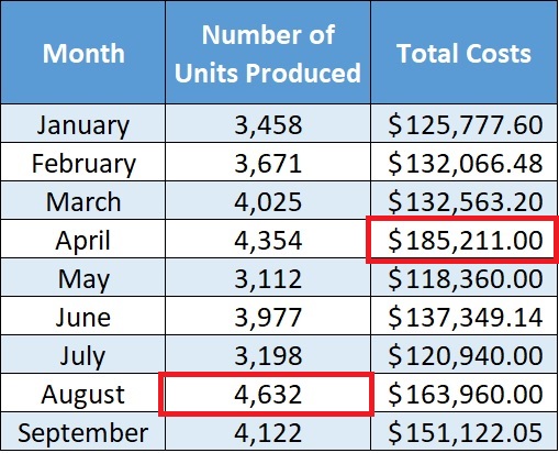
In cases such as the one above, it is important to remember that the high-low values should be based on units (e.g. number of units produced) and not on the total costs.

As such, our highest value for this set of data will be 4,632 in units and $163,960 in total costs.

Next, we find the lowest value.

As highlighted above, our lowest value is 3,112 in units and $118,360 in total costs.

Now we compute for the variable cost per unit:

Variable Cost Per Unit = (HAC – LAC) ÷  (HAU – LAU)

= ($163,960 – $118,360) ÷ (4,632 – 3,112)

= $45,600 ÷ 1,520

= $30.00

Now that we have our variable cost of $30.00, we can compute for the fixed cost:

Fixed Cost = HAC – HAVC

= $163,960 – (4,632 x $30)

= $163,960 – $138,960

= $25,000

 

We can also use the other formula to compute for the fixed cost:

Fixed Cost = LAC – LAVC

= $118,360 – (3,112 x $30)

= $118,360 – 93,360

= $25,000

As expected, either formula results in the same total fixed cost of $25,000.

You then communicate to the manufacturing company that based on the data they sent, their variable cost per unit is $30.00 and their fixed cost is $25,000.

Always remember that when you’re using the high-low method, the high-low values should be based on units and not the total costs.

Exercise#3

We gathered the following data:

We will be using the high-low method to segregate the variable and fixed costs.

First, we need to identify and highest and lowest values:

Highlighted in green is the lowest value with an activity level of 2,545 units and $42,950 total costs.

Highlighted in red is the highest value with an activity level of 4,915 units and $83,235 total costs.

Now that we have our high and lowest values, we can compute for the variable cost per unit:

Variable Cost Per Unit = (HAC – LAC) ÷  (HAU – LAU)

= ($83,235 – $42,950) ÷ (4,915 – 2,545)

= $40,285 ÷ 2,370

= $17.00

Now that we have our variable cost per unit ($17.00), let’s proceed to the next step which is computing for the fixed cost:

Fixed Cost = HAC – HAVC

= $83,235 – (4,915 *$17)

= $83,235 – $83,545

=  -$310

As per computation, we get a negative fixed cost. This is invalid, and we need to redo our computation.

Negative Fixed Cost

When the fixed cost formula results in a negative fixed cost, that means that either or both of the highest and lowest values aren’t representative of the set of data.

As can be seen from the set of data above, the highest value is at 4,915 units and $83,235 total costs.

Notice that its total costs far exceed the other values.

The next highest total cost is $58,350, which is a $24,885 difference.

Compared to other values which only have about $500 to $5,000 difference between them, the difference between the highest and second highest values is very high.

As such, it can be considered that the highest value is an outlier.

We will then have to use the second-highest value to correct the computation:

Highlighted is the second-highest value with an activity level of 4,085 units and $58,350 total costs.

Let’s compute once again for the variable cost per unit, this time with the updated values:

Variable Cost Per Unit = (HAC – LAC) ÷  (HAU – LAU)

= ($58,350 – $42,950) ÷ (4,085 – 2,545)

= $15,400 ÷ 1,540

= $10

And with that, we can proceed to the computation of fixed cost:

Fixed Cost = HAC – HAVC

= $58,350 – (4,085 x $10)

= $58,350 – $40,850

= $17,500

Using the high-low method, we gather that the variable cost is $10 per unit, and the total fixed cost is $17,500.

Limitations of the high-low method

The high-low method’s simplicity is its main advantage as well as its biggest limitation.

Because it only uses two values from a set of data, extreme values at that, it ignores the other values in the computation for variable and fixed costs.

Thus, it is best used if there is a linear relationship between cost and activity.

As it does not consider all the values within the set of data, it might not be a good representation of a business’s cost and volume behavior.

For that, it’d be better to use activity-based costing (ABC).

The high-low method also does not take into account any changes within the costs (e.g. increase in the price of raw materials, rent, etc.).

It assumes that cost will remain the same in the future.

This can be remedied by redoing the computation if there are any changes within the costs.

Another limitation of the high-low method is that it does not consider the impact of inflation.

This can be somewhat remedied by adjusting the values for inflation before you start the computation using the high-low method.

Lastly, the extreme values (highest and lowest) used by the high-low method may happen to be outliers.

Meaning that they don’t represent the set of data.

This could happen if the two activity levels are far too apart, or if a significantly high cost is incurred at the highest level.

There is a work-around for outliers though.

If either or both the lowest and highest values do not represent the set of data, you may use the next best value (e.g. second lowest or second highest).

The high-low method is a quick and simple way to segregate variable and fixed costs.

However, because of its limitations, it’s best to not over-rely on it.