Wrapping Text in Google SheetsLearn how to wrap text in Google Sheets


While Google Sheets is commonly used to store numerical data such as monthly sales or expense reports, some people use it to manage huge chunks of text.
For example, a Google Sheet document may contain the training manual of a company, a strategic plan, or maybe even a project tracker.
Documents such as these will, more often than not, contain more text values than number values.
Now, entering text in Google Sheets isn’t exactly the same experience as doing it in Word.
When you enter text in a cell in Google Sheets, by default, any text that does not fit within the cell will spill over the adjacent empty cell.
Emphasis on empty.
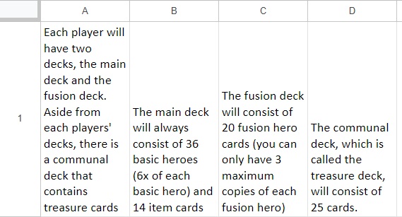
This is because if the adjacent cell isn’t empty, this will happen:
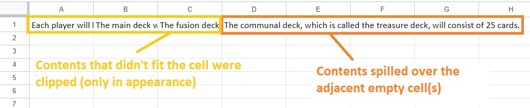
If the adjacent cell isn’t empty, the contents that don’t fit the cell will be clipped.
This means that only the contents that fit the cell will appear. It wouldn’t be an issue if you don’t have to show all the text content of a cell (such as in the case of URLs).
But if you need to have all the contents appear (such as in training manuals), this just won’t do.
So you question yourself, is there a solution to this issue? Well, yes. There is a solution. You just need to change the text wrapping settings of the concerned cells.
In this article, I’ll be showing you how to wrap text in Google sheets so that all the contents of the cell show.
I’ll also be showing you some tricks you can do to make text blocks in Google Sheets more readable.
Let’s get started.
Wrap Text in Google Sheets Via the Format Menu
For the first method of wrapping text in Google Sheets, we’ll be using the Format menu.
This menu allows the user to change the format of the selected cell or cells (such as the cell’s number format, text alignment, etc.).
What we’re interested in this menu is the option to change the Wrapping setting of the selected cell or cells.

Here’s how we can wrap text in Google Sheets via the format menu.
How to wrap text in Google Sheets
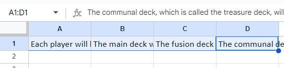
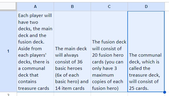
- Select the cell or cells that contain text that we want to wrap.
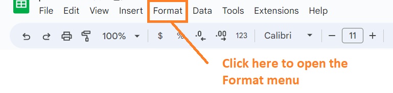
- Open the Format menu by clicking on “Format” on the menu bar (as shown in the illustration below).
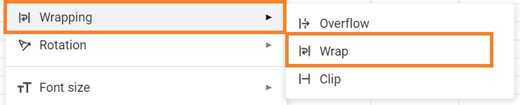
- With the Format menu opened, hover the mouse over “Wrapping”.
- We should now see three Wrapping options: (1) Overflow (default wrapping setting), which spills the contents that don’t fit the cell over the adjacent empty cell or cells, (2) Wrap, which will wrap the text in the cell, and (3) Clip, which will clip the contents that don’t fit the cell (only in appearance). Since we want all the text contents of the cell to appear, we will be selecting “Wrap” (click on it).
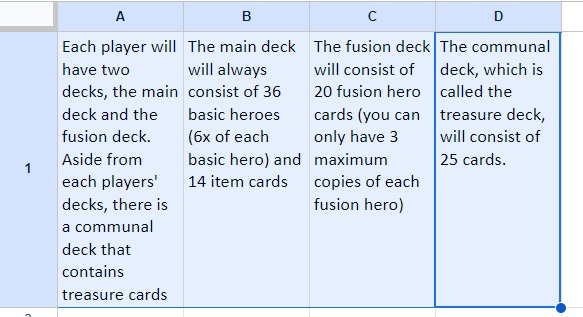
- This will wrap the text in the selected cells (as can be seen below).
All the text contents now appear within their respective cells.
To accommodate this, Google sheets will automatically adjust the cell height to fit all the text.
Text wrapping is dependent on the width of the cell. If we increase the cell width, Google Sheets will adjust the cell height so that the text contents fit the cell as lean as possible.

Wrap Text in Google Sheets Via the Toolbar
A quicker method to wrap text in Google Sheets is using the toolbar (which we can find just below the menu bar).
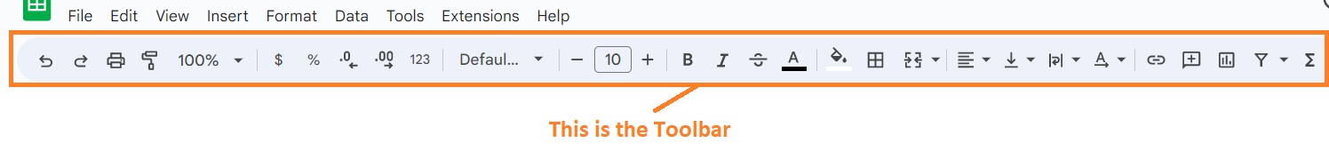
In this toolbar, we should see a button that allows us to change the text wrapping settings of the selected cell or cells.
We refer to this as the Text wrapping button.
Let’s use this button to wrap the text in certain cells:
How to wrap text in Google Sheets
- Select the cell or cells that contain text that we want to wrap.
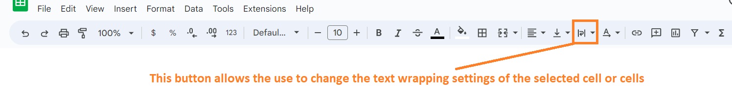
- Click the Text wrapping button which can be found on the Toolbar.

- We should now see three options: (1) Overflow (leftmost option), which spills the contents that don’t fit the cell over the adjacent empty cell or cells, (2) Wrap (middle option), which will wrap the text in the cell, and (3) Clip (rightmost option), which will clip the contents that don’t fit the cell (only in appearance). Since we want all the text contents of the cell to appear, we will be selecting “Wrap” (click on it).
- We should now see all the text contents within the cell (or cells) appear. Google Sheets will automatically adjust the cell height to fit the contents in the cell as lean as possible.
This method requires fewer clicks than the first method, yet it still yields the same result (which makes it my preferred method of wrapping text in Google Sheets).
Manually Wrap Text in Google Sheets With a Keyboard Shortcut
In the previous text wrapping methods, Google sheets will automatically wrap text in cells based on cell width.
However, what if you want more control over how to wrap text?
Google Sheets allows that too via line breaks. The keyboard shortcut to insert a line break is Ctrl + Enter (or Alt + Enter).
Here’s how you can have more control over how to wrap text in Google sheets.
How to wrap text in Google Sheets
- Select the cell that contains the text that you want to wrap.
- Press F2 to enter cell edit mode.
- Move the cursor to where you want to enter a line break. Then, press the keyboard shortcut Ctrl + Enter (or Alt + Enter). Do this for every line break that you want to insert.
Adding a line break will separate the text before and after it and ensures that they appear on separate lines. This effectively wraps the text without having to depend on the cell’s width.
The main drawback of this method is that you can only do it cell-by-cell. If you have a lot of cells that need text wrapping, this can get very time-consuming. But if you really need to have more control over how to wrap text, then this method is the best for you.
Wrap Text in the Google Sheets App
If you have to wrap text in Google sheets via the app, you can still do so.
Here’s how:
- Select the cell that contains the text that you want to wrap. You can also select an entire row or column. (The thing with working with the app is that there is less control over how you select cells (e.g. you cannot select two or more cells unless you’re selecting an entire row or column)
- Tap the Cell/Text Format It’s represented by an A with several horizontal lines icon (as shown below).

- Open the Cell tab. You should see an option to toggle “Wrap text”. Tap it to wrap text within the selected cells (or cells in the case of entire rows or columns).

This should wrap the text within the selected cell or cells.
Change Text Alignment to Make Text More Readable
In Google Sheets, the default text alignment is bottom-left.
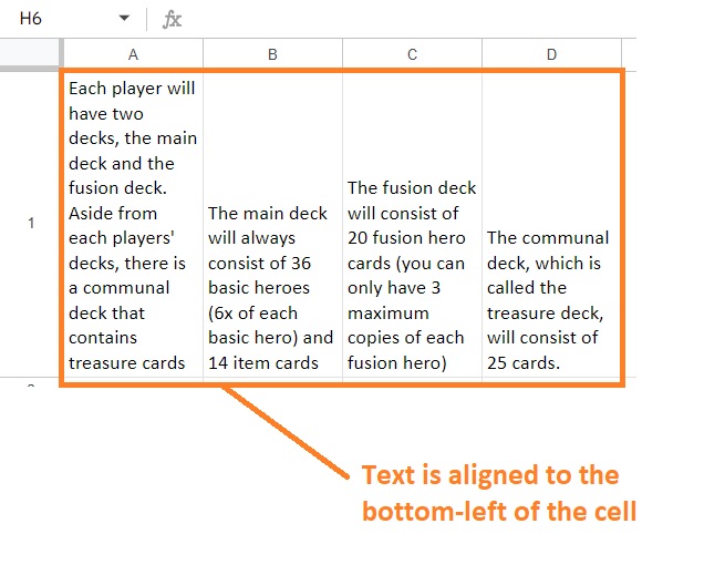
There’s nothing inherently wrong with this alignment setting as you can still read the text contained in the cell just fine. But it could be better.
When you read a book, how is the text aligned? Isn’t it aligned to the top-left of the page? So why not align the text in Google Sheets the same? That way, it’ll be like you’re reading a book.
Here’s how to change the text alignment of a cell or cells in Google Sheets:
- Select the cell or cells that you want to change the text alignment
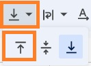
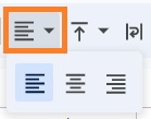
- In the toolbar, you should find the Vertical align button (as shown below).

- Clicking this button will give you three vertical alignment options: (1) Top, which will align the text to the top of the cell, (2) Middle, which will align the text to the vertical center of the cell, and (3) Bottom, which will align the text to the bottom of the cell (and also the default setting). Click the Top option.
- This should align the text to the top-left of the cell. This makes the text easier to read.
You can also change the horizontal text alignment. There is a Horizontal align button that will let you change the horizontal alignment of text in the selected cell or cells.

Clicking this button will present you with three horizontal alignment options: (1) Left, which will align the text to the left side of the cell, (2) Center, which will align the text to the horizontal center of the cell, and (3) Right, which will align the text to the right side of the cell.
Conclusion
And those are the ways you can wrap text in Google Sheets. Wrapping text in Google Sheets makes long text strings easier to see and read.
Which of the method do you prefer the most? Let me know in the comments.