Use Wildcards With VLOOKUP in ExcelMake VLOOKUP more flexible by using wildcard characters

Last Updated: February 10, 2023

Written By:
Patrick Louie

Reviewed By:
FundsNet Staff

Excel’s VLOOKUP function is one of the most used functions in Excel. And I say deservedly so.

The utility it provides is undeniable. It makes working with data much easier.

It can help you get your desired data from a table or a range of cells without having to look at the cells one by one.

However, despite its greatness, VLOOKUP still has its limitations.

One issue with VLOOKUP is that cannot find or fetch a value if there’s a difference in the lookup value.

This isn’t a problem if you know the complete lookup value. But if you only know a portion of it, VLOOKUP may not give you your desired result.

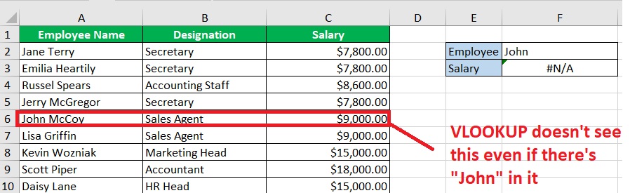
For example, let’s say that you’re looking at a list of employees with their respective designations and salaries.

You want to find out the salary of “John”, but you forgot his full name.

Still, you try to use VLOOKUP to find out John’s salary. Note that the list spells out the full name of the employees.

That being the case, VLOOKUP will return an #N/A value because it cannot find a cell in the list that exactly contains the lookup value “John”.

Fortunately, there’s a way to circumvent this issue. And that’s with the help of wildcard characters (*,?).

With wildcard characters, you can make VLOOKUP function properly even with a partial lookup value.

In this article, you’ll be learning how to use these wildcards when using Excel’s VLOOKUP function.

Let’s get started.

The Wildcard Characters

In Excel, there’s a total of 3 wildcard characters that you can use: *,?,~.

Asterisk (*) – this wildcard character substitutes for any number of characters (number or text). If it’s placed after a text (e.g. John*), VLOOKUP will search for a value that starts with the text (e.g. John McCoy). If it’s placed before a text (e.g. *Terry), VLOOKUP will search for a value that ends with the text (e.g. Jane Terry). You can also enclose a text with asterisks (*John*), then VLOOKUP will search for a value that has the text (e.g. John Kevin Doe, Mary John Spears)
Question Mark (?) – this wildcard character substitutes for any one character; for example, if you use “P?ay” as the lookup value, VLOOKUP may search for the text “Pray” or “Play”. Each question mark (?) substitutes one character
Tilde (~) – this wildcard character does not substitute for anything. Rather, it nullifies the effects of the other two wildcard characters if placed direct before either of them. For example, if you want to look up the value “Any*”, your lookup value should be “Any~*” to nullify the effect of the asterisk (*)

VLOOKUP and the Asterisk (*)

In this section, I’ll be showing you how the asterisk (*) wildcard character with VLOOKUP.

The asterisk (*) substitutes for any number of characters. It is usually used with a text or number string to make searches even with a partial lookup value.

VLOOKUP with lookup value that starts with a particular text or number string

Let’s go back to our first example above:

Here, you wanted to find out the salary of “John”. However, VLOOKUP returned an #N/A value because it didn’t find an exact match.

You can circumvent this by using the asterisk (*) wildcard. You just need to place it after the string (e.g. John*)

To do so, you’ll have to modify the VLOOKUP formula. It should be this:

=VLOOKUP(F2&”*”,A1:C11,3,0)

Here, the lookup value is set to F2&”*”. F2 is a cell reference to the name of the employee.

We use an ampersand (&) to concatenate the cell reference with the wildcard character *.

With this, VLOOKUP will search for a value that starts with the value in cell F2 (e.g. John McCoy).

VLOOKUP with lookup value that ends with a particular text or number string

Now, let’s say that you know the last name of the employee but not his/her first name.

You can also use the wildcard asterisk to make VLOOKUP search even with a partial lookup value. Let’s use the same dataset:

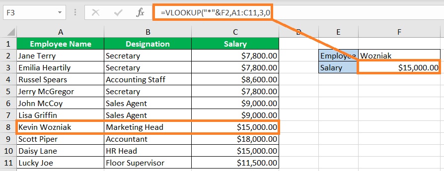
This time, you know of an employee that has the last name “Wozniak”.

To make VLOOKUP work properly, you have to modify the formula into this:

=VLOOKUP(“*”&F2,A1:C11,3,0)

Here, the lookup value is set to “*”&F2. F2 is a cell reference to the name of the employee.

We use an ampersand (&) to concatenate the cell reference with the wildcard character *.

With this, VLOOKUP will search for a value that ends with the value in cell F2 (e.g. Kevin Wozniak).

VLOOKUP value that includes a particular text or number string

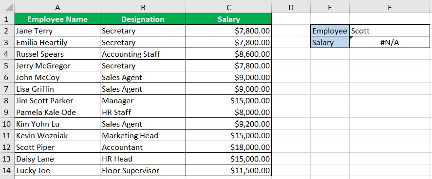
Suppose you know the middle name of the employee but don’t know his/her first or last name.

We can make VLOOKUP search for a matching value by enclosing the name between two asterisks.

For example, let’s say that you want to find out the salary of the employee with the middle name “Scott”.

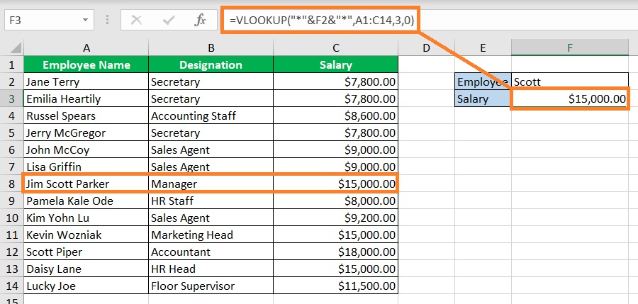
To make VLOOKUP work properly, you need to modify the formula into this:

=VLOOKUP(“*”&F2&”*”,A1:C14,3,0)

Here, the lookup value is set to “*”&F2&”*”. F2 is a cell reference to the name of the employee.

We use an ampersand (&) to concatenate the cell reference with the wildcard character *.

With this, VLOOKUP will search for a value that contains the value in cell F2 (e.g. Jim Scott Parker).

Tips when using *

The VLOOKUP formula when you want to search a value that starts with a particular text or number string is =VLOOKUP(value&”*”,table_array,col_index,0). value refers to the text or number string, or cell reference, table_array refers to the range where VLOOKUP searches, and col_index is the column placement of the resulting value
The VLOOKUP formula when you want to search a value that ends with a particular text or number string is =VLOOKUP(“*”&value,table_array,col_index,0)
The VLOOKUP formula when you want to search a value that includes a particular text or number string is =VLOOKUP(“*”&value&“*”,table_array,col_index,0)
Asterisk (*) replaces any character, including spaces

VLOOKUP and the Question Mark (?)

The question mark (?) wildcard character substitutes for one character.

It’s usually used with a text or number string.

For example, let’s say that you’re working on this dataset:

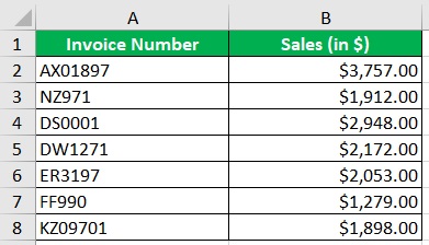
It’s a list of invoices with their sales amount. Each invoice number starts with a random two-letter combination.

After that is the actual number. Now, what if you only want to use the number part of the invoice number as the lookup value? This is what happens:

VLOOKUP returns an #N/A value. This is because there is no cell that exactly matched “1271”.

To circumvent this, you’ll have to use the wildcard character “?”. The VLOOKUP formula will be modified to this:

=VLOOKUP(“??”&E2,A2:B8,2,0)

This formula will search and match for a value that starts with exactly two characters before the lookup value (invoice number in this case).

Use the question mark (?) wildcard character to substitute one character of any text or number string (including spaces).

VLOOKUP and the Tilde (~)

The tilde (~) wildcard character nullifies the effect of the other wildcard characters (*,?).

This is useful if the lookup value uses any of the two characters.

For example, let’s say that your lookup value is “IGN*”.

If you use this as the lookup value as is, VLOOKUP will search and match the first value it finds that starts with the string IGN.

For example, in this dataset:

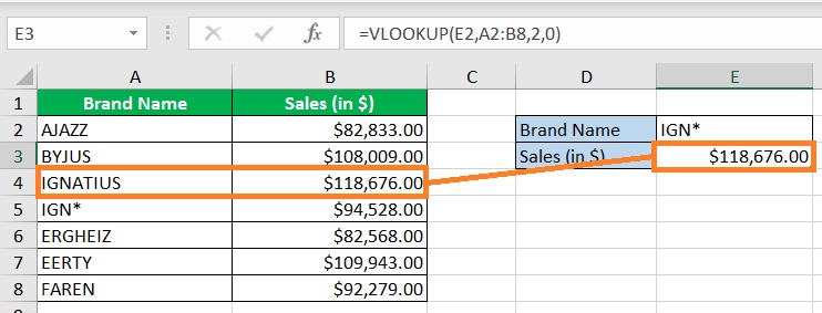
VLOOKUP finds the value “IGNATIUS” first (which starts with “IGN”).

But you want to know the sales of IGN*.

To do so, you’ll have to use a tilde (~) to nullify the effect of the asterisk (*).

And there. The resulting value matches with the “IGN*”.

Conclusion

And those are the ways you can use wildcard characters to make VLOOKUP more flexible.

Two of the wildcard characters serve to substitute characters in a string, while one serves to nullify the effect of the other two.

Are you able to make more use of VLOOKUP? Let me know in the comments.