Two Easy Ways to Combine First & Last Names in Microsoft ExcelTwo Methods for Easily Combining Multiple Words or Text into a Single Cell

Last Updated: February 9, 2023

When working with spreadsheets, organizing the names in distinct columns is often convenient for the user, specifically when it comes to organizing the first and last names.

It is easier to do work when establishing and organizing the names in different columns.

However, there are times when you must combine the first name and last name in a single column depending on how you want to present your data.

Luckily, doing this manually is not necessary.

In Excel, there are two methods that make it easy to combine two to three or more words or text into a single cell.

We will see in this tutorial what these two methods are.

First & Last Names Merging Formulas

We can practice two formulas in Excel by combining the first and last names into a single cell.

We will tackle this in an easy step-by-step process.

Method of Ampersand (&)

In this method, we will see how ampersand (&) works.

It is mostly used to combine word threads into one.

To merge your first name and last name, this is exactly how it works.

Assume the following set of first names and last names:

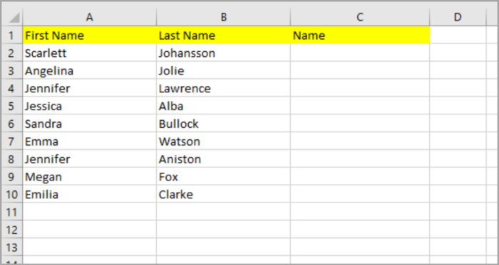
Steps in merging the first names and last names using the ampersand (&):

Highlight/select the designated cell where you choose to appear (C2) the combined text.
Then type the sign equal (=).
Click the A2 cell which contains the first name, then follow it using the ampersand (&).
Click the B2 cell which contains the last name corresponding to the first name (A2).
Hit the Enter Key.
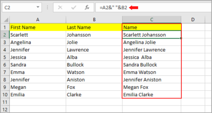
The first and last names are now combined together, then again without space sandwiched between them. You can change it by adding spaces between the formulas. After the first name cell reference, add & “ “. The formula will now be shown as =A2&” “&B2.
The first name and last name with a space sandwich in between are now combined into a single cell (C2). Copy this to the rest of the formula in column (C) by double-clicking the fill button (located at the right bottom area of cell C2).

Each row now contains the full names of all the cells in column C3.

The Function of CONCATENATE ()

The CONCATENATE () function and the ampersand (&) operator have the same function.

The main difference between the two is in the way they are used.

Steps in merging the first names and last names using the CONCATENATE () Function:

Highlight/select the designated cell where you choose to appear (C2) the combined text.
Then type the sign equal (=).
Go to function and select CONCATENATE and follow it by typing opening bracket.
Click the A2 cell which contains the first name, then follow it using a comma (,).
In adding space between the first name and last name, input the symbol double quotes (“ “).
Click the B2 cell which contains the last name. This is now our sample formula: =CONCATENATE(A2,” “, B2).
Hit the Enter Key.
The first name and last name with a space sandwich in between are now combined into a single cell (C2). Copy this into the rest of the formula in column (C) by double-clicking the fill button (located at the right bottom area of cell C2).

Important Notes:

If you prefer the arrangement of the last name first followed by a comma (,) and then the first name, reverse the order of A2 and B2. Then add the comma symbol in between the double symbol quote. This is now our sample formula: =CONCATENATE(B2,” , “,A2).
You can use any type of symbol in separating the first name and last name.
If there are three cells given with the arrangement for the first name, middle name/middle initial, and last name with the cells A2, B2, and C2 in the destination for cell D2, you can simply add the additional cell in the formula between the first and last name. Now, the formula for this type of format in the D2 cell is =CONCATENATE(A2,” “,B2,” “,C2).
If there are three cells given with the arrangement for the first name, middle initial, and last name with cells A2, B2, and C2. Now, the formula for this type of format in the D2 cell is = CONCATENATE(A2,IF(B2=””,” “,”&LEFT(B2,1)&”.”),C2).

The function LEFT() is the number of how many words there are in the cell and specifies what number you will take.

The number corresponds to the arrangement of words in the given cell, ranging from one to how many letters there are in the middle initial.

For the middle name, we will take the first letter(#1) because we need the initial (first letter) of the middle name.

Then input the space and dot operators. And lastly, for the C2 cell (last name), we also need it to be concatenated.

Now by using this formula, the value of the first name and last name is now dependent and will be the result of the value of the original cell.

If there are changes in the original value, it will also be changed in the combined value.

Since this is a formula, there will be an error in your result (combined name/column) if you wish to delete the entire A column and B column (this is where the first and last names are located).

You can see the error in the picture below.

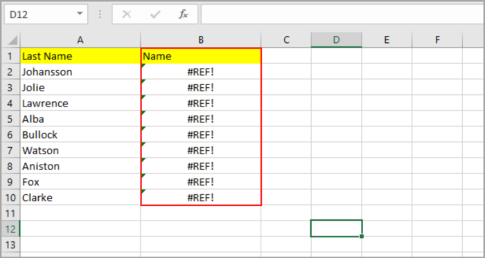
This is because you deleted the A column and B Column which means that the inputs in the formulas are now nonexistent.

To prevent this, the easiest way to do this is to copy this by right-clicking the combined values and selecting the Paste Option, then selecting the Values(V) in the option.

The formulas of the combined values are now permanent values.

See the sample in picture format below:

You can now delete the A column and B column as you wish.

Combining First & Last Names by Flash Fill Function

There are techniques in Microsoft Excel that take advantage of the program’s pattern recognition abilities.

This is called Flash Fill functionality and is available on the versions of Microsoft Excel 2013 onwards.

Here is the step-by-step process of how to combine the first name and last name by using Flash Fill:

Select the first cell where you want to combine the first names and last names in the column to appear.
Then manually type the first name and last name of the subject.
Go to the Data tab, you will find the Flash Fill button in the Data tool group then click it. For the shortcut, you can do this by pressing CTRL+E (for Windows) and Command+E (for Mac).

This method is fast and easy and will duplicate the same format in all the cells in the column.

Also, this method doesn’t need the typing and writing of formulas.

And in most cases, this is quick, reliable, and precise.

In other scenarios, punctuation and capitalization are present in your work.

This method also works in this kind of situation.

If you were given the first name and last name with all small letters, the capitalization of the first letter of the first and last names is easy and simple when using Flash Fill.

It will also automatically copy it into the rest of the cells in the column.

Customizing the pattern or arrangement in this method can also be done easily.

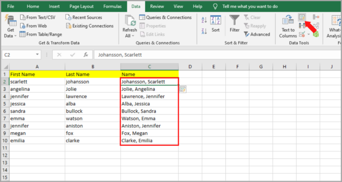
Whether your preferred arrangement of names is the last name, then followed by a comma (,), and lastly followed by the first name, the original column doesn’t affect the outcome of the Flash Fill if you try to edit or remove it because the method doesn’t need a formula to operate.

Therefore, removing permanently the two original columns doesn’t affect the combined names of the first name and last names, respectively.

Conclusion

Given the first name and last name located in two different columns, we showed you how to combine them in single, different patterns using two ways in Excel in this tutorial.

And having said that, there are other ways of combining two different names or even words.

There are other ways of combining the given words located in different columns. TEXTJOIN function (only in new versions) and VB scripts are other examples.

But the two methods that we tackle in this tutorial are the two simplest and most commonly used methods in Excel.

We hope that these demonstrations help you in your project.