Rounding Up or Down to the Nearest 5 (or Any Multiple) in ExcelLearn how to round off numbers to the nearest 5 (or any multiple) in Excel


You may sometimes have to round numbers up or down to simplify the data that you’re working on.
Sometimes, you may have to approximate values to a certain multiple (e.g. 5, 10, 15, etc.).
Thankfully, you can use functions in Excel to perform these tasks.
You don’t have to round off each one by one.
And yes, there’s a function for simply rounding off a number to the nearest 1.
There’s also a function for rounding off a number to a certain integer or multiple.
Now when we say round off a number (or value) to the nearest multiple, say 5, we mean that we’re approximating the value to a multiple of 5.
For example, let’s say we have the number 19.
If we are to round it off to a multiple of 5, we can either round it up to 20 or round it down to 15 since these are the nearest multiples of 5.
Since 19 is closer to 20 than 15, we will be rounding up 19 to 20.

If you were to round down a number to the nearest multiple, you’d always end up with a number that is lower than the original number.
On the other hand, if you were to round up a number to the nearest multiple, you’d always end up with a number that higher than the original value.
In Excel, rounding off, rounding down, and rounding up to the nearest multiple each have a specific function.
We will be learning how to use these functions so that you can round any value to a certain multiple anytime you have to.
Use the MROUND Function to Round to the Nearest 5 (or Any Multiple)
With the MROUND function, we can round a number (or value) to the nearest multiple of another value (e.g. nearest 5, 10, 25, etc.).
The formula for using this function is straightforward. Here it is:
=MROUND(number, multiple)
Where
value – refers to the number or a reference to the cell that contains the number that you want to round
factor – refers to the multiple of which the value will be rounded to (e.g. multiple of 5, 10, 15, etc.)
So if you want to simply round off 22 to the nearest multiple of 5, then the formula will be =MROUND(22,5).
If you want to round off the number in cell A2 to the nearest multiple of 10, then the formula will be =MROUND(A2,10).
How to Use MROUND
For illustration purposes, we will be using the following dataset:

Your task here is to round the number to the nearest 5.
To do so, you’ll be using the MROUND function.
- Select a blank cell where the rounded number will show. Ideally, you’d want this cell to be adjacent to the cell that contains the number that you want to round. (For our illustration, we will be selecting cell B2).
- In the selected cell, enter the formula for the MROUND function. Since you’re rounding the number to the nearest multiple of 5, make sure to set the factor to 5. (For our illustration, the formula will be =MROUND(A2,5)).

- Press the Enter key to execute the function. The selected cell should now show a rounded value of the number.

- Copy the formula to the rest of the column (until the next empty row).
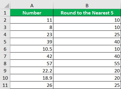
You’ll notice some of the numbers have decimals.
Thankfully, the MROUND function works for both decimals and integers. You can also set a decimal as the factor (or multiple).
Use the FLOOR Function to Round Down to the Nearest 5 (or Any Multiple)
The MROUND function rounds a number to the nearest multiple. It will either round up or round down the number depending on whether it is nearer to the lower or upper bound.
If you want to always round down a number to the nearest multiple, you may want to use the FLOOR function instead.
Unlike the MROUND function, the FLOOR function always rounds down a number to the nearest multiple.
The formula for using the FLOOR function is as follows:
=FLOOR(value,significance)
Where
value – refers to the number or a reference to the cell that contains the number that you want to round down
significance – refers to the multiple of which the value will be rounded down to (e.g. multiple of 5, 10, 15, etc.)
Since the FLOOR function always rounds down a number, it will never return a value that is greater than the number.
If we use the FLOOR function on the number 28 with a significance of 5, it will return a value of 25.
In contrast, if we use the MROUND function on the number 28, it will return a value of 30.
How to Use FLOOR
For illustration purposes, we will be using the following dataset:

Your task here is to round the number down to the nearest 5. To do so, you’ll be using the FLOOR function.
- Select a blank cell where the rounded-down number will show. Ideally, you’d want this cell to be adjacent to the cell that contains the number that you want to round down. (For our illustration, we will be selecting cell B2).
- In the selected cell, enter the formula for the FLOOR function. Since you’re rounding down the number to the nearest multiple of 5, make sure to set the significance to 5. (For our illustration, the formula will be =FLOOR(A2,5)).

- Press the Enter key to execute the function. The selected cell should now show a rounded-down value of the number.

- Copy the formula to the rest of the column (until the next empty row).

Similar to the MROUND function, the FLOOR function works on both integers and decimal numbers.
Here’s a side-by-side comparison of the results of MROUND and FLOOR functions, highlighting the different results.

Use the CEILING Function to Round Up to the Nearest 5 (or Any Multiple)
The CEILING function is functionally the opposite of the FLOOR function.
Rather than always rounding down a number, the CEILING function always rounds up a number instead.
For example, use the CEILING function to round up the numbers 21 and 24 to the nearest multiple of 5, both numbers will be rounded up to 25.
If we were to use the MROUND function on these numbers, the number 21 will be rounded down to 20 while the number 24 will be rounded up to 25.
The CEILING function is useful if you always want to round up a number to the nearest multiple. The formula for using the CEILING function is as follows:
=CEILING(value,significance)
Where
value – refers to the number or a reference to the cell that contains the number that you want to round up
significance – refers to the multiple of which the value will be rounded up to (e.g. multiple of 5, 10, 15, etc.)
How to Use CEILING
For illustration purposes, we will be using the following dataset:

Your task here is to round the number up to the nearest 5.
To do so, you’ll be using the CEILING function.
- Select a blank cell where the rounded-up number will show. Ideally, you’d want this cell to be adjacent to the cell that contains the number that you want to round down. (For our illustration, we will be selecting cell B2).
- In the selected cell, enter the formula for the CEILING function. Since you’re rounding up the number to the nearest multiple of 5, make sure to set the significance to 5. (For our illustration, the formula will be =CEILING(A2,5)).

- Press the Enter key to execute the function. The selected cell should now show a rounded-up value of the number.

- Copy the formula to the rest of the column (until the next empty row).
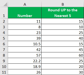
Just like the previous two functions, the CEILING function works on both integers and decimal numbers.
Here’s a side-by-side comparison of the results of MROUND and CEILING functions, highlighting the different results.

Use the ROUND, ROUNDUP, and ROUNDDOWN Functions to Round to the Nearest 5 (or Any Multiple)
While the ROUND, ROUNDUP, and ROUNDDOWN functions are mainly used to round decimal numbers to the nearest integer, we can also use them to round numbers to the nearest multiple. They’re not as straightforward as the previous functions though.
The formula to do so is as follows:
=ROUND(value/multiple,0)*multiple
Where
value – refers to the number or a reference to the cell that contains the number that you want to round
multiple – refers to the multiple of which the value will be rounded to (e.g. multiple of 5, 10, 15, etc.)
For example, let’s say we want to round the number 24 to the nearest multiple of 5 using the ROUND function.
The formula for doing so will be =ROUND(24/5,0)*5. This will give the result as if using the MROUND function.
If you want to round down the number, replace ROUND with ROUNDDOWN. If you want to round up the number, replace ROUND with ROUNDUP.
Conclusion
And those are different functions you can use to round a number to the nearest 5 (or any multiple).
I hope that you’ll be able to use your learnings here in your future endeavors.