How to Reverse the CONCATENATE Function in ExcelHow to Split the Contents of a Cell into Separate Cells


In Excel, there’s the nifty CONCATENATE function that combines the contents of two or more cells and put them into one cell.
This is really useful when you find that values that were supposed to be in one cell were split into separate cells when the data was imported into Excel.
With just a simple formula, you can combine the values that were split into separate cells.
Here’s an example of what the CONCATENATE function does:

What I did here is combine the content in cell A1 with cell B1 by using the CONCATENATE function. I put a “ “ in between the cells.
This is so that there’s a space between the content in cell A1 (first name) and the content in cell B1 (last name). The result is “John Smith”.
But, what if you want to opposite?
By that, I mean splitting the contents in one cell into separate cells.
Can you still use the CONCATENATE function to do that? Well, obviously not. But is there a dedicated reverse CONCATENATE function in Excel? Unfortunately, such a thing doesn’t exist yet.
However, that doesn’t mean that you can’t do it in Excel.
There are several methods that you can use in Excel that will help you perform the opposite of the CONCATENATE function.
And in this article, I’ll be showing you how you can do each one.
By the end of the article, you should be able to reliably split the contents of a cell into separate cells.
Ready to learn? Well, let’s get started then!
Use a Formula to Perform a Reverse CONCATENATE
For the first method, we’ll be using a formula that will split the contents of a cell into separate cells.
To better explain it, let me show you an example.
Here we have a dataset with names separated by commas.
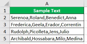
What I want to do here is to split each name in each cell into cells of their own.
To do so, I’ll be using the following formula:
=TRIM(MID(SUBSTITUTE($A2,”,”,REPT(” “,999)),COLUMNS($A:A)*999-998,999))
I’ll be entering this formula into cell C2:

When I press the Enter key, the first name in cell A2 should appear:

Next, I’ll copy the formula for each name in the dataset. This will be the result:
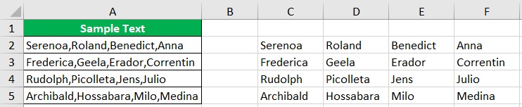
I have successfully split the names into separate cells.
The Formula
Let’s talk about the formula I used to split the contents:
=TRIM(MID(SUBSTITUTE($A2,”,”,REPT(” “,999)),COLUMNS($A:A)*999-998,999))
In this formula, there are three variables. These are the following:
![]()
![]()
$A2 – this refers to the first cell of the range from which you want to split contents. Be sure to prefix it with a dollar sign ($) to make an absolute reference to the column. If the first cell of the range is cell B2, then this variable will be $B2
“,” – this refers to the separator of the values. In the illustration above, the names are separated by a comma, which is why I used a “,” here. If the separator is a space, this will variable will be ” “.
$A:A -this refers to the column of the first cell of the range. Be sure to prefix it with a dollar sign ($)
Use Flash Fill to Perform a Reverse CONCATENATE
For the second method, we’ll be using Excel’s Flash Fill feature to perform a reverse CONCATENATE. What Flash Fill does is automatically fill up cells according to the pattern that it senses. Flash Fill is available in the 2013 and later versions of Excel.
Now, let’s use this dataset (a list of names) to illustrate how we can use the Fill Handle to perform a reverse CONCATENATE:
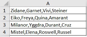
To create a pattern the Flash Fill will recognize, we will enter the first name of the first cell in the adjacent cell (to the right):
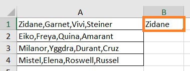
That should be enough for Flash Fill to recognize. Let’s see if it works. With the cell selected (the one where we entered the pattern), press the keyboard shortcut Ctrl + E to run Flash Fill:
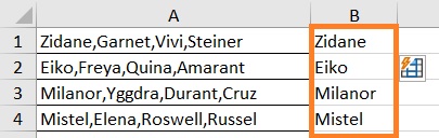
And it did! It successfully separated the first name in each cell into its own cell. Now let’s try it again with the second name in the first cell:
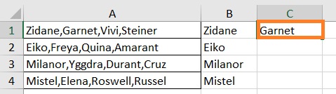
Let’s try Flash Fill again if it still works:
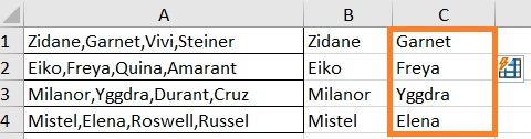
And it still does! Now we do this for every name in the cell to split all names in the cell into separate cells:

And there we have it. We have successfully performed a reverse CONCATENATE with Flash Fill.
Things to note with Flash Fill
The thing with Flash Fill is that it may not work every time. If the pattern is too complicated for Flash Fill to recognize, it may not function properly. It works best when the pattern is simple, and the cells in the column are similarly structured.
Use Text to Columns to Perform a Reverse CONCATENATE
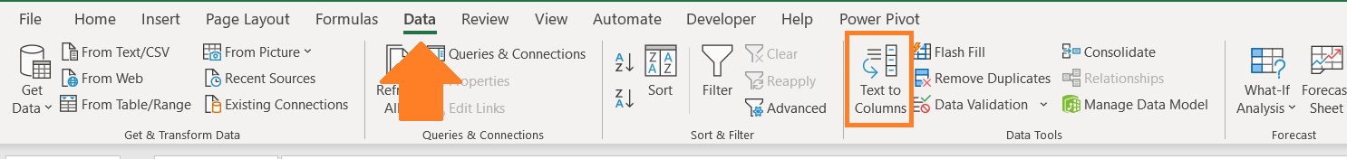
For the last method that we’ll be discussing in this article, we’ll be using Excel’s Text to Columns feature.
This nifty feature can be found on the data tab. In the middle section of the ribbon, you should see the Text to Columns button.
The great thing about Text to Columns is that you can select more than one separator/delimiter.
For example, let’s try to split the contents of this dataset into separate cells:

As can be seen, the values in each cell are separated by different delimiters. But not to worry.
We can still split these values with the Text to Columns feature.
First, select the cells that contain the contents that we will be splitting.
Then, click the Text to Columns button (which can be found on the Data Tab). This will open the Convert to Text Columns Wizard.
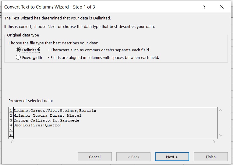
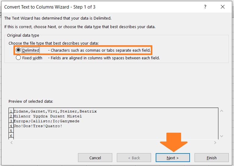
For step 1 of the Wizard, we are to choose between two options: Delimited and Fixed Width.
Since we want to split contents that are separated by delimiters, we’ll be choosing the Delimited option. Then we’ll click the Next button.
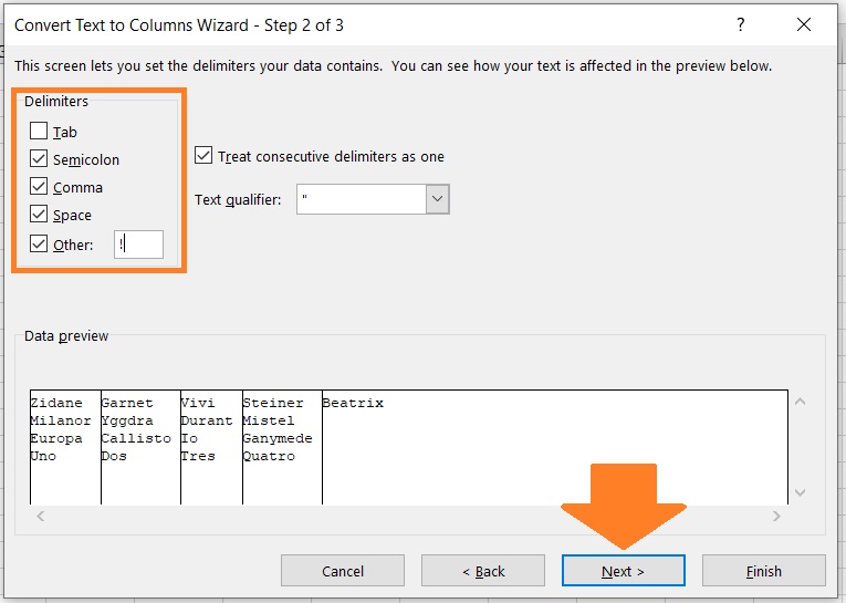
For step 2 of the Wizard, we’ll be specifying what our delimiters are, which are the following: comma (,), space ( ), semi-colon (;), and exclamation point (!).
We’ll then click the Next button.
For the last step of the Wizard, we are given the option to choose the data format of each column, as well as where the result will appear.
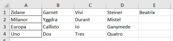
But for now, we’ll leave things as is and just click the Finish button.

And we have successfully split the contents into separate cells.
Things to Note
The one thing you have to be careful with using Text to Columns is that it directly modifies the original data.
If you want to retain the original data, I suggest that you make a copy of the sheet before using Text to Columns.
Conclusion
And those are the different ways you can perform a reverse CONCATENATE in Excel.
You should be able to reliably to split the contents of any cell into separate cell.
Which of the three method do you prefer the most? Let me know in the comments.