Remove Decimals in ExcelHere are several methods to remove decimals in Excel
When you’re often working with numbers, you’d inevitably come across decimals.
They’re the numbers that come after a dot or period.
For example, let’s say the number 100.34.
Here, there is a decimal of .34.
Decimals represent a number that isn’t quite whole (like an integer).
Working with decimals is necessary if your work requires your data to be as detailed as possible.
But if just presenting the whole numbers (or integers) is enough, you might just want to remove them (the decimals).
Doing so makes the data relatively easier to read.
I mean, isn’t 14 easier to read than 14.03?
In this article, we will be learning different methods to remove decimals from numbers in Excel.
One method does not involve any rounding of numbers as it only extracts the whole number.
The rest will involve rounding up or down numbers. Let’s get started.
Use the TRUNC Function to Remove Decimals in Excel
Let’s go first with the method that doesn’t involve rounding off.
In this method, we’ll be using the TRUNC function.
What this function does is take a decimal and truncate it to a specific length.
For example, you can use it to set decimals to always show two numbers.
Of course, we can also use this function to remove decimals entirely.
The formula to use the TRUNC function is as follows:
=TRUNC(number,[num_digits])
Where:
number – refers to a numerical value or cell that contains the number that you want to truncate (or extract the whole number from)
num_digits – this is where you will specify the precision of the truncation. This is optional and has a default value of 0. Not assigning a value here will automatically remove any decimals.
Remove Decimals Using the TRUNC Function
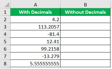
Suppose we have the following dataset:

Your task is to remove decimals from the dataset.
There’s no need to round off numbers. As such, the TRUNC function is perfect for this task.
- Select a blank cell, ideally next to the cell that contains that number that you’ll truncate. In our illustration, this will be cell B2.
- Enter the formula for the TRUNC function in the selected cell. Press the Enter key after doing so. For our illustration, the formula will be =TRUNC(A2).

- The cell should now show a number that doesn’t have decimals.

- Copy the formula to the rest of the column (until the next empty row).

As you can see, the TRUNC function simply removed the decimals. It didn’t round off the numbers.
Format Cells to Remove Decimals in Excel
The next method we’ll be using doesn’t involve the use of a formula.
Rather, we’ll be directly working on the original data.
We won’t be needing another cell or column to show the results.
In this method, we’ll be formatting the cells that contain the decimal numbers.
Remove Decimals by Formatting Cells
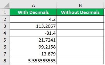
We’ll be using the following dataset for illustration:

Your task is to remove decimals by formatting the cells that contain them.
- Select the cells that contain the decimal numbers. If they’re all in the same column, you can simply select the column instead. In our illustration, we’ll be selecting column A.
- Right-click anywhere on your selection. Select Format Cells from the options. This will open the Format Cells dialog box.

- In the Format Cells dialog box open the Number tab. Select Number from the Category menu. Then, on the box after Decimal places, enter 0 (zero). Click the OK button after doing so.

- That dataset should now contain numbers that don’t have decimals. The numbers will also be rounded off to the nearest integer. (e.g 5.5555 will be rounded up to 6).

- Alternatively, rather than using the Format Cells dialog box, you can use the Decrease Decimal button. You can access it by opening the Home tab. It will be located somewhere in the middle of the tab. Repeatedly click on it until all decimals within your selection are removed.
![]()
This method only changes how the values look. The original can still be seen if you click on the cell and press F2 or look at the formula bar.
Use the INT Function to Remove Decimals in Excel
For the next method, we will be using the INT function.
What this function does is similar to the TRUNC function.
It extracts only the integer (whole number) part of a decimal number.
It also always rounds down the number. So 11.6 and 11.11 will both return a value of 10 when you use the INT function.
Finally, it will always return an integer value, unlike the TRUNC function where you can specify how many decimal places there will be.
The formula for using the INT function is as follows:
=INT(number)
Where:
number – refers to a numerical value or cell that contains the number that you want to truncate (or extract the whole number from)
Remove Decimals Using the INT Function
We’ll be using this dataset again for illustration:

Your task is to remove decimals from the dataset. This time, you’ll have to use the INT function.
- Select a blank cell, ideally next to the cell that contains that number that you’ll remove decimals from. In our illustration, this will be cell B2.
- Enter the formula for the INT function in the selected cell. Press the Enter key after doing so. For our illustration, the formula will be =INT(A2).

- The cell should now show a number that doesn’t have decimals.

- Copy the formula to the rest of the column (until the next empty row).

Take note of how the INT function interacts with negative numbers. Since it rounds down, it will make any negative number more negative.
For example, a value of -13.279 will be rounded down to -14 after you apply the INT function.
Use the Round Function to Remove Decimals in Excel
If you want more control over how to round off numbers, you might want to use the ROUND function instead of the INT function.
The ROUND function has three variants: ROUND, ROUNDDOWN, and ROUNDUP. The ROUND function rounds up or rounds down to the next nearest integer.
So with ROUND, 10.1 will be rounded down to 10 and 10.71 rounded will be rounded up to 11.
The ROUNDDOWN variant always rounds down the number no matter the value of the decimal. On the other hand, the ROUNDUP variant always rounds up the number.
The formula to use the ROUND function is as follows:
=ROUND(value, )
Where:
number – refers to a numerical value or cell that contains the number that you want to round off
num_digits – this is where you will specify the number to which you want to round. Assigning a value of 0 (zero) here will automatically remove any decimals.
For the ROUNDDOWN or ROUNDUP variants, just replace the “ROUND” in the formula.
Remove Decimals Using the ROUND Function
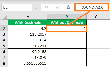
We’ll be using the following dataset for illustration:

Your task is to remove decimals using the ROUND function.
- Select a blank cell, ideally next to the cell that contains that number that you’ll round off. In our illustration, this will be cell B2.
- Enter the formula for the ROUND function in the selected cell. Press the Enter key after doing so. For our illustration, the formula will be =ROUND(A2,0).

- The cell should now show a number that doesn’t have decimals.

- Copy the formula to the rest of the column (until the next empty row).

The ROUND function is a more versatile function than the INT function when it comes to rounding off numbers.
If you want more control over how to round off numbers, the ROUND function is the better choice.
Conclusion
And those are several ways to remove decimals in Excel.
Select the method that suits your preference the best.
You should now be able to remove decimals from any Excel workbook whenever you have to.
