Remove Dashes (-) in ExcelHere are two easy ways to remove dashes (or hyphens) in Excel

When you work with a dataset in Excel, you may sometimes come across text or number values that have dashes (or hyphens) in them.

This is common for particular types of numbers such as SSNs (social security numbers), passport numbers, phone numbers, etc.

That’s fine. But what if you want to remove these dashes because you only want the numbers to show?

Well, you can always remove the dashes manually. But as you’d expect, that would take time especially if the data is large.

Besides, you’re working with Excel here. There are always more efficient ways of doing things. And yes, that includes removing dashes.

So if you’re planning to remove those dashes from your dataset, read on.

We will be discussing several methods of removing dashes in Excel.

By the end of the article, you should be able to easily remove dashes from any datasets that you work on (if you want to).

Let’s get started.

Use the Replace Function to Remove Dashes in Excel

The first method we’ll be discussing involves using the Replace function (actually, the Find and Replace function).

What this does is find any cell within the sheet (or workbook) or selection that has your specified parameter (which is the value you input in the textbox after “Find what”).

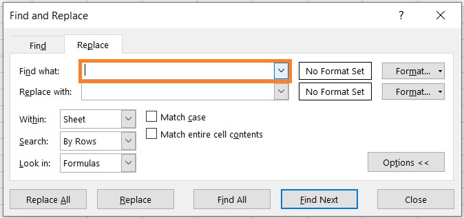
It will then replace the values in the cells with your specified new value.

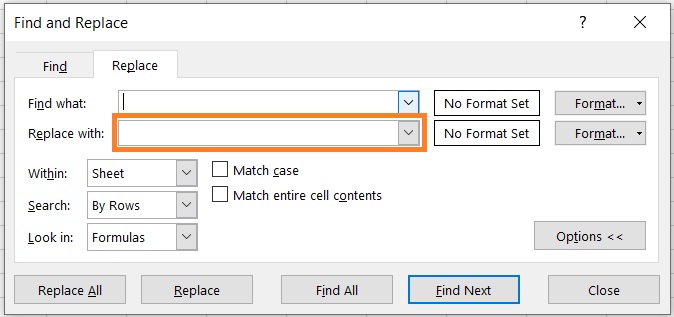
You can replace each cell one by one or you can replace all of them.

We can use this nifty function to remove dashes in a dataset. What we’ll do is replace the dashes (-) with a null or blank value.

How to Use the Replace Function to Remove Dashes in Excel

We will be using the following data for our illustration:

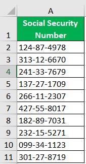
• Select the dataset that you want to remove dashes from. If it’s the entire sheet, you can skip this step. For our illustration, we will be selecting cells A2 to A11.
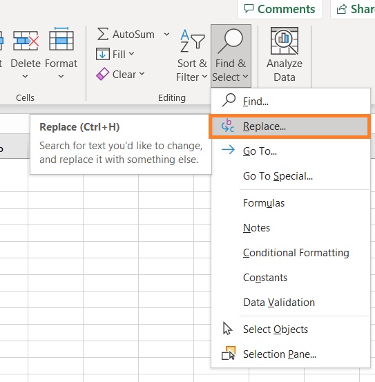
• Press the key combination CTRL + H to open the Find and Replace dialog box. Alternatively, you can access this dialog box from the Home tab. You’ll find a Find & Select button. Click on it and select the Replace option.

• Go to the dialog box. In the textbox after “Find what”, type the dash symbol (-).

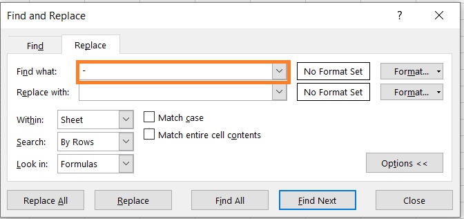
• Leave the textbox after “Replace with” blank. This will essentially delete the dashes within your selection.

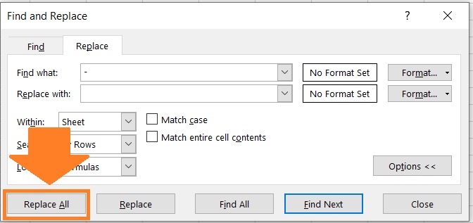
• Click the Replace All button. (If you want to remove the dashes one by one, you may click the Replace button instead).

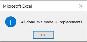
• Excel will inform you how many replacements it made. Click the OK button.

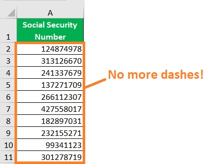
• You will notice that the dashes within your selection are now removed.

Things to To Take Note Of When Using This Method

Using the replace function is a quick and easy way to remove dashes in Excel. However, there are things you need to be wary of when using it:

• It works on your original data. This means that it will apply the changes to the original data set. If you want the original data to remain untouched, it’s recommended that you make a backup copy of the file before using the replace function.
• If the values from which dashes will be removed are numbers, any leading zero will be removed. This is because Excel, by default, automatically removes leading zeros from any number value. You can format the cells to always show a certain length of numbers if you have to.
• Using the Replace All button will remove all dashes from your selection, even ones that you don’t want to be removed. If you have dashes that you don’t want to remove, you can use the Replace button instead.

Use the Substitute Function to Remove Dashes in Excel

Similar to the Replace function, the SUBSTITUTE function replaces a certain value with a new value that the user specifies.

Unlike the Replace function though, you can only access the SUBSTITUTE function using a certain formula, which is as follows:

=SUBSTITUTE(cell, “old value”,“new value”)

Where:

cell – refers to the cell that contains the data from which you want to replace values

old value – refers to the value that you want to replace

new value – refers to the value that you want to replace the old value with

What we can do is “substitute” the dashes with a blank or null value.

How to Use the SUBSTITUTE Function to Remove Dashes in Excel

We’ll be using the same data for our illustration:

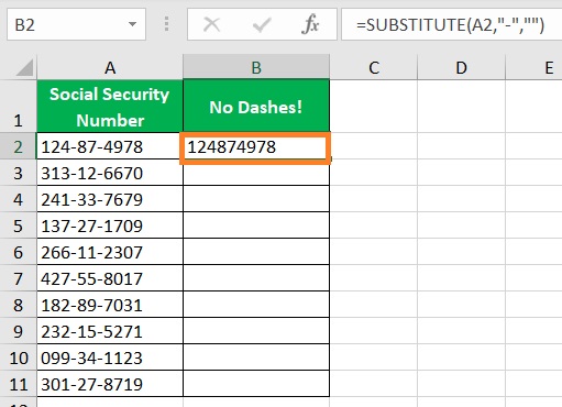
• Select an empty cell, preferably adjacent to the cell that contains the value from which you’ll remove dashes. In our example, we will be selecting cell B2.

• In the selected cell, type the formula for the SUBSTITUTE function. In our example, the formula will be =SUBSTITUTE(A2,“-”,“”). What you’re doing here is replace the dashes within the selected cell with a blank or null value.

• Press the ENTER key. The function will return the value in cell A2 with no dashes.

• Copy the formula and paste it to the cells in the column until the next empty row.

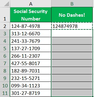
• You should now have a column of values that don’t have dashes.

Things to Take Note Of When Using This Method

Do note that when you’re using this method, the result will show in another cell (unlike with Replace function which changes the original data).

By default, the value in the cell will be treated as text.

As you can see from our illustration above, the result is aligned to the left as if it’s a text string.

This is also the reason why leading zeros appear by default. If you want these values to be treated as numbers, you’d have to format the cells that contain them.

Conclusion

In this article, you were able to learn of two methods to remove dashes in Excel.

Both are accessible methods and have their quirks.

The Replace function replaces the original data.

On the other, the SUBSTITUTE function shows the result in another location.

Feel free to use whichever method suits your needs or situation.

I hope that you find this article useful!