How to Remove Commas in Excel (from Numbers or Text String)Here are various ways to Remove Commas in Excel

Commas. Such a wonderful thing (especially in language).

They make certain sentences different with or without their presence.

For example, while the sentences “Let’s eat grandma!” and “Let’s eat, grandma!” have the same string of words, they don’t mean the same thing.

This is why they always say that commas are important.

In Excel where sentences are sparse, commas often serve a different function.

For one, they make large numbers (those ranging from 1,000 and up) more readable.

Let’s say that a cell has 2917828 in it and the one next to it has 2,917,828.

Which of the two is easier to read as a number?

It’s probably the one with the commas, right?

Another purpose for commas is to separate related values in the same cell.

For example, a cell contains the first and last names of a person.

In this case, the name is Rudy Spears.

To make it more pronounced which is the first name and which is the last, we can add a comma to separate them.

So rather than simply Rudy Spears, the cell will instead contain Rudy, Spears.

This makes it easier to identify which is the first name, and which is the last.

In some cases though, you might want to do away with commas.

By that, I mean that you may want to clean your Excel sheet of unnecessary or unwanted commas.

The most obvious way to do this is to manually edit the cells where you want to remove commas.

However, this can become unnecessarily time-consuming and tedious if the data you’re dealing with is huge.

Fortunately, there are various efficient ways to remove commas in Excel.

In this article, we will learn how to remove commas in Excel using various techniques.

Remove Commas Using the Find and Replace Functions

The first method we’ll be using to remove commas involves the use of two functions: Find and Replace.

The Find function searches for any cell within your selection that has the value that you selected.

On the other hand, the Replace function replaces the specified value in any cell within your selection and replaces it with a new value that you specify.

 

The nifty thing about these functions is that you can use them for the whole Excel sheet, workbook, or a selection of cells. They’re easy to use too.

How to Remove Commas Using the Find and Replace Functions

For illustration purposes, we will be using the following data:

Suppose we want to remove the commas in column B (Age and Gender) so that the format become (Age) (Gender) rather than (Age), (Gender). We’ll be using Find and Replace to remove these commas.

• Select the cells where we want to remove the commas. In this case, we will be selecting column B. (If you want to select the entire sheet instead, you can press Ctrl + A or click on the upper right corner of the sheet).

• On the Home tab, click the Find & Select button. By default, it’s located on the rightmost side. Clicking on it will present us with some options.

Click “Replace”. This will open the Find and Replace Dialog Box.

Alternatively, you can press Ctrl + H on your keyboard. Doing so will open the Find and Replace Dialog Box

• In the input field next to “Find What”, input the comma (,) symbol. This communicates to Excel that we want to find any cell within the selection that contains a comma.

• In the input field next to “Replace with”, leave it blank. Alternatively, if you want to replace commas with a space, then input space in the input field.

• The final step is to click the “Replace All” button. This should remove the commas in all of the cells that contain them within our selection.

And the result? No more commas!

Remove Commas Using the Substitute Function

Another method to remove commas is to use the Substitute Function (via a formula).

What this function does is it replaces the value in the cell with the new value that you specify. The formula for the Substitute function looks like this:

=SUBSTITUTE(CELL,“(value to be replaced)”,“(new value)”

For example, if we want to change “Any” to “All” in cell A1, our formula will be:

=SUBSTITUTE(A1,“Any”,“All”)

Similar to the Replace function, we can use the Substitute function to remove commas.

The difference is that the result will be shown in a different cell.

How to Remove Commas Using the Substitute Function

In this illustration, we will use the following data:

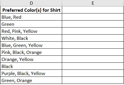
Suppose that we want to remove all the commas in column D but we don’t want to touch the data within it.

Rather, we want to input the result in column E. We will do so by using the Substitute function:

• Select the first of the blank column (which is cell E2 in this case). This is where we will first input the formula to perform the substitute function.
• Input the formula =SUBSTITUTE(D2,“,”, “”). This should replace the comma in cell D2 with a blank.

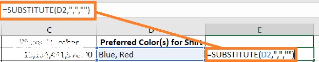
• Press the Enter key, and voila! No more commas!

• The next step is to apply the formula to the rest of the column. There are two ways to do this. The first is to copy the formula and paste it on the rest of the column. The other is to double-click the fill handle in the bottom right corner of cell E2.

Remove Commas Using the NUMBERVALUE Function

The next step of removing commas only applies to cells that contain numerical values or numerical data that is formatted as text.

We do this by using the NUMBERVALUE function (via a formula).

What this function does is that it converts the data within the selected cell into a number that has no commas.

Do note that if the destination cell has formatting that includes commas, this will not work.

The formula to use the NUMBERVALUE Function is as follows:

=NUMBERVALUE(Cell or Number or Value)

For example, if we want to get the NUMBERVALUE of cell A1, the formula will be:

=NUMBERVALUE(A1)

Similar to the Substitute function, we will be needing another column to show the results.

How to Remove Commas Using the NUMBERVALUE Function

For illustration purposes, we will be using the following data:

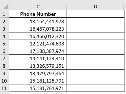
We want to remove the commas in Column C using the NUMBERVALUE function.

We will be using Column D to present the results:

• Select the cell where you want to perform the NUMBERVALUE function. In this case, the cell will be cell D2.
• Input the formula =NUMBERVALUE(C2). This will result in the numerical value of cell C2 without the commas.

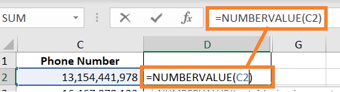
• Press the Enter key. The result should be as follows:

• The next step is to apply the formula to the rest of the column. There are two ways to do this. The first is to copy the formula and paste it on the rest of the column. The other is to double-click the fill handle in the bottom right corner of cell E2.

Remove Commas Using the Text to Columns Function

Another method to remove commas is to use the “Text to Columns” function. Not only can this function remove commas, but it can also separate the related values by columns.

For example, you have a cell that contains the first and last names of a person, separated by a comma.

Using the “Text to Columns”, you can separate the first name and last name into two different columns.

How to Remove Commas Using the Text to Columns Function

We will be using the following data for illustration:

We want to separate the first and last names into two columns. To do so, we will be using the Text to Columns function:

• We might want to ensure first that there are enough blank columns next to the one that we’ll be working with. In this case, we already have column B blank.
• Select the columns that you want to remove the commas. In this, we will select column A.
• On the Data tab, click the “Text to Columns” button. It should be located somewhere in the middle of the toolbar.

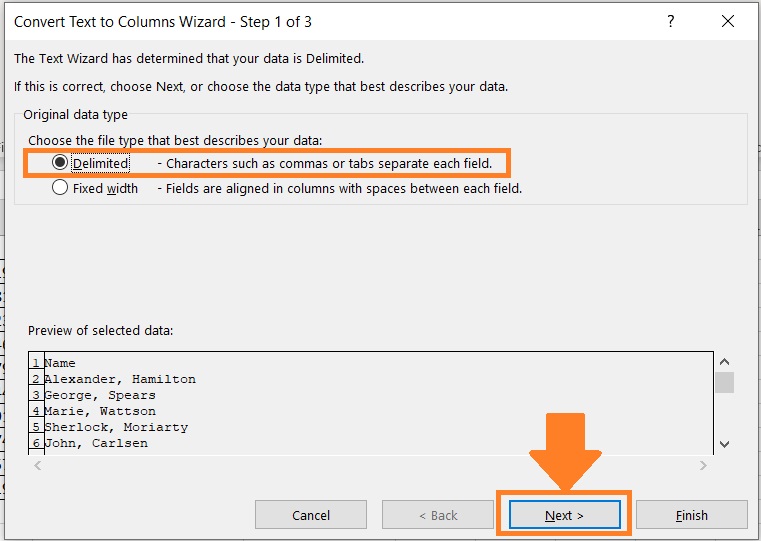
• This will open the “Convert Text to Columns” wizard. We will be taking 3 steps in this wizard. Step 1 of 3 is to choose the file type. We want to use delimited so we will select it. Then we click the next button.

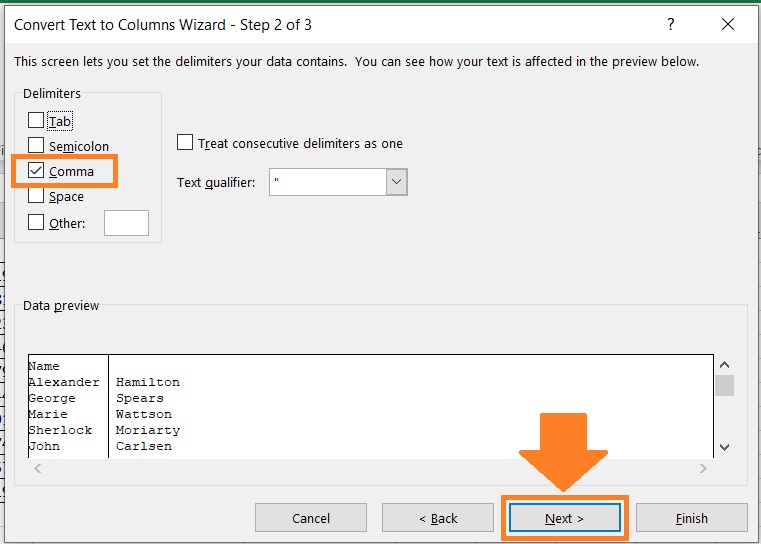
• Step 2 of 3 of the wizard is to select the delimiter contained in our data. Select “Comma” on the delimiter options. Then we click the Next button.

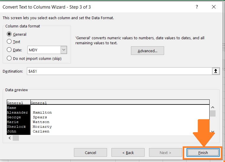
• Step 3 of 3 of the wizard is to select the destination column. By, this will be on the column that you’re working on. So really, all we need to do here is to click the Finish button.

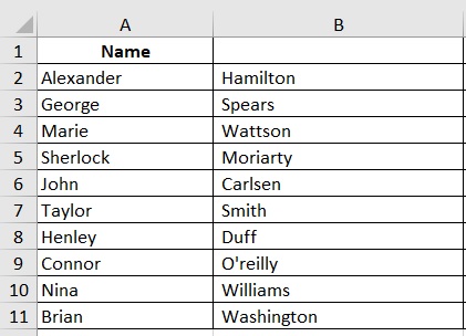
• The result should look like this (no more commas and names are separated into different columns):

Remove Commas from Formatted Cells

None of the methods above will work if the cell that you’re working on (or destination cell in the case of the NUMBERVALUE function) is formatted to contain numbers that have commas.

Most probably, the data contained in the cell doesn’t have commas.

They’re just formatted to look like that.

Take a look at this:

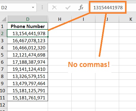
On the cell, the number has commas. But if we take a look at the formula bar, there are no commas.

So using Replace or Substitute will not remove the commas in this case.

What we need to do is to format these cells so that they don’t contain commas.

How to Remove Commas from Formatted Cells

• Select the cells that you want to remove commas. In this case, it will be the cells in column D.
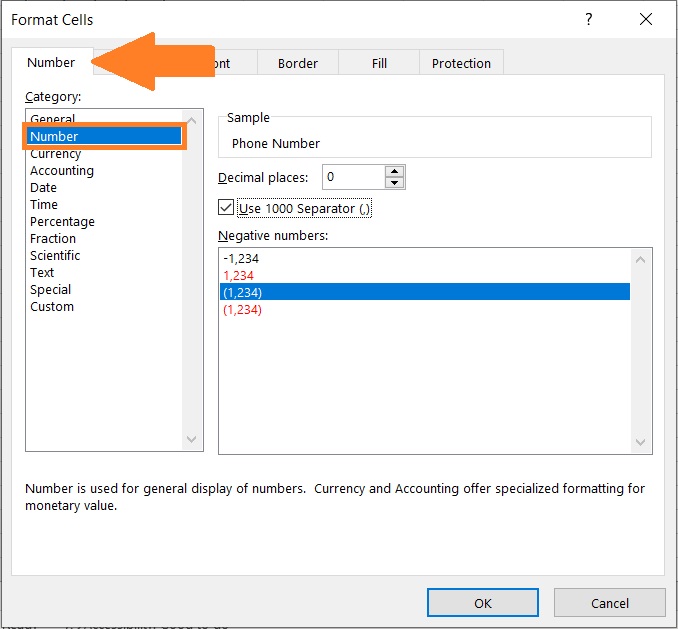
• Right-click on the selection. This will present us with various options. Click “Format Cells”. This should open the Format Cells dialog box.

• On the number tab, navigate to the number category.

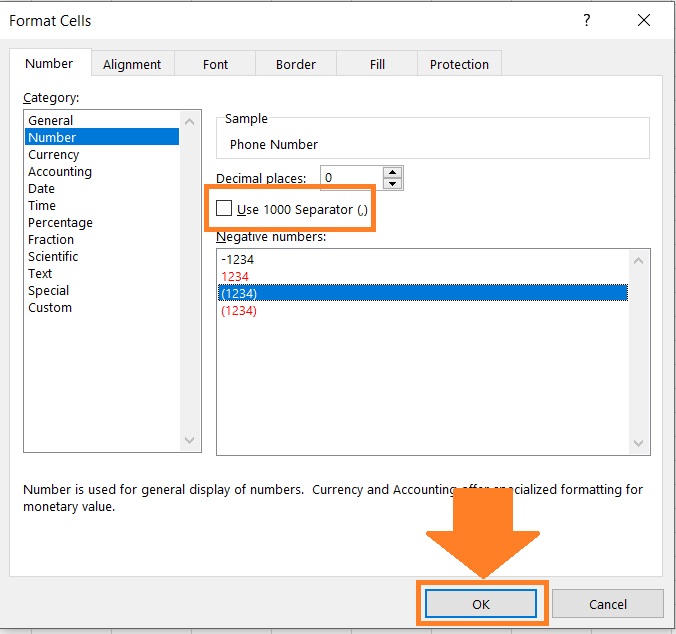
• Make sure to untick the check box beside “Use 1000 separator (,)”. Then click the OK button.

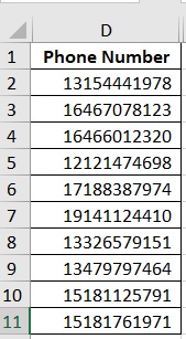
• This should format the selected cell to contain numbers that have no commas.

Conclusion

And those are the various method that you can use to remove commas in Excel.

I hope that you find this article useful!