Make Leading Zeros Appear in ExcelLearn how to add leading zeros in Excel

When you enter a number in Excel, you’d notice that any leading zeros will disappear when you press the Enter key.

For example, say you enter 01710 into cell A. After you press the Enter key on your keyboard, it will appear as 1710 instead, removing the leading zero.

This happens because Excel automatically truncates any leading zeros from a number (i.e. numerical value).

It makes sense. After all, you write it as 1 + 1 and not as 01 + 01.

The zero before the number does not have value and only serves to unnecessarily lengthen the number. Normally, leading zeros aren’t necessary when it comes to working with numbers.

I say normally because there will be situations where you need those leading zeros to show.

For example, you have to use Excel to record sales invoices.

If you’re familiar with what a sales invoice looks like, you’ll know that some invoices may have leading zeros to their sales invoice number (i.e. SI#). As such, you want Excel to show these leading zeros.

Other examples would be phone numbers, zip codes, social security numbers, etc.

But again, Excel will remove any leading zeros from a number by default. What are you supposed to do in such situations?

In this article, we’ll be discussing just that. I’ll show you how to make leading zeros appear in Excel whenever you need to.

Let’s get started.

Add an Apostrophe (‘) Before the Number

For the first method, we’ll be using a special character: the apostrophe (‘). It has a special function in Excel.

If it appears as the first character of a string, it will prompt Excel to treat the rest of the string as text.

It doesn’t matter if the string only contains numbers. So long as the apostrophe appears as the first character, the string will be treated as text.

Thus, we can use it to make leading zeros appear. Excel no longer treats the number as a “number” but instead treats it as text.

Thus, Excel will not remove any leading numbers. For example, instead of entering 01710, we enter ‘01710 instead.

This method works great if you’re just about to enter the number(s).

Though, you can still use it if the numbers are already in the worksheet.

You just need to edit the numbers individually, making sure that they start with an apostrophe then add the leading zeros before the number.

Remember that this method converts the numbers to text.

Thus, some mathematical functions (e.g. SUM) will assign a zero (0) value to these ‘numbers’.

Change the Cell Format to Text

Another method that works best when you’re just about to input the number into the worksheet involves changing the cell format to text.

While this method still works for numbers that are already in the worksheet, just like with the previous method, you’d have to individually edit the number to add the leading zeros.

To change the cell format to text, you have to:

• Select the cells where you want to apply the text format (to make the leading zeros appear). For example, I want cells A1 to A25 to show leading zeros.

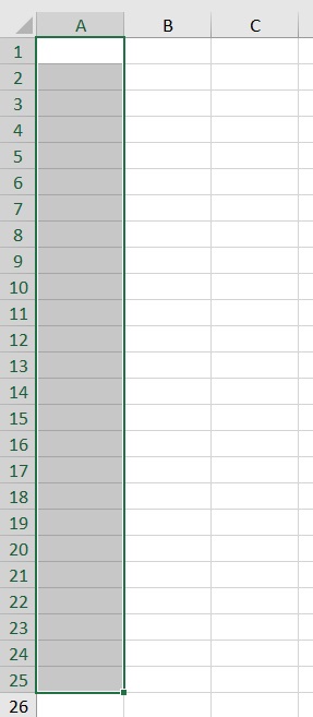
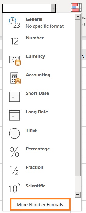
• Open the Home tab. In the middle of the ribbon, you should find the Cell Format box (it will show General by default). Click the dropdown arrow in the box.

• A list of Cell Format options will appear. Select More Number Formats from among them. This will open the Format Cells dialog box.

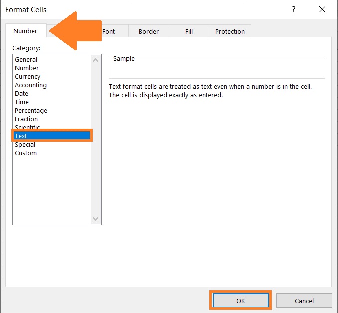
• In the dialog box, open the Number tab. Under Category, select Text. Then, click the OK button.

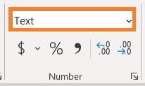
• This should change the cell format of the selected cells to Text.

• Now, any values that are entered into the selected cells will always be treated as text. Thus, if we enter a number with leading zeros into one of these cells, they should now appear.

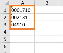
Remember that this method converts the numbers to text. Thus, some mathematical functions (e.g. SUM) will assign a zero (0) value to these ‘numbers’.

Apply Custom Format to Make Leading Zeros Appear

This next method is the one I recommended the best. Just like the previous method, we’ll be changing the format of the cells that contain or will contain the numbers with leading zeros.

However, instead of changing the format to Text, we’ll be using a custom format.

What I like about this method is that it works whether you’re just about to enter the numbers or the number are already in the worksheet.

And it does not convert the numbers into text, which means that mathematical functions will work on them just fine.

To apply a custom format to make leading zeros appear, here are the steps:

How to Make Leading Zeros Appear

• Select the cells where you want to apply the text format (to make the leading zeros appear). For example, I want cells A1 to A25 to show leading zeros.

• Open the Home tab. In the middle of the ribbon, you should find the Cell Format box (it will show General by default). Click the dropdown arrow in the box.

• A list of Cell Format options will appear. Select More Number Formats from among them. This will open the Format Cells dialog box.

• Open the Number tab. Then, under Category, select Custom.

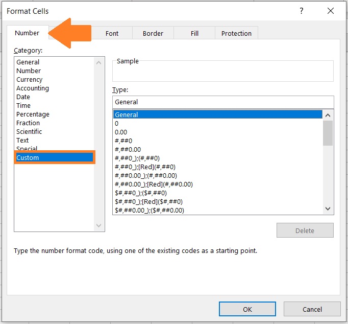
• On the right side of the dialog box, there’s a textbox that is below “Type”. This is where we’ll enter the custom format. For now, I want the selected cells to always show 5-digit numbers (we’ll expound on this later). To do so, I’ll enter 00000 (five zeros) in the textbox. Then, I’ll click the OK button.

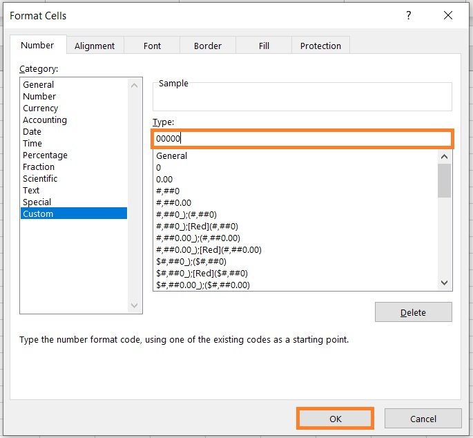
• The custom format should now be applied to the selected cells. To test, let’s enter numbers with different numbers of digits.

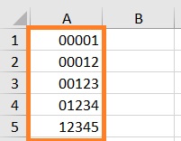
As seen above, numbers that have less than five digits will have leading zeros. These numbers are still considered numbers. As such, mathematical functions will work on them just fine.

0s and #s

Let’s expound on the custom format. For numbers, we have two placeholders: 0 and #.

When you use 0 as a placeholder, leading zeros will appear depending on the set length of the number.

For example, if the custom format is set to 00000, any number on that cell will always appear with 5 digits.

If the number only has 2 digits (e.g. 12), the cell will add leading zeros to make the number show 5 digits (e.g. 00012).

Now, if we only want to add one leading zero to any number, then only use one 0 as a placeholder, then set the rest as #.

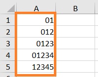
For example, the cell has a custom format of 0####. What this does is add one leading zero to any 4-digit or below number. Here’s a visual representation:

Add Leading Zeros Using Formula

For this section, I’ll be showing you the formulas that you can use to add leading zeros to numbers.

The CONCATENATE Function

The concatenate function combines two or more strings into one.

For example, if we concatenate the strings “00” and “123”, the cell will show “00123”. Thus, we can use this function to add leading zeros to numbers.

The formula to use the CONCATENATE function to add leading zeros is as follows:

=CONCATENATE(­­text_1, text_2)

Where

text_1 – is the leading zero/s. If you want to add one leading zero, then set it to 0. If you want to add two leading zeros, set it to 00, and so on and so forth.

text_2­ – refers to the number or cell that contains the number

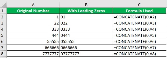
Here’s a visual representation of how the formula works:

The REPT and LEN Function

The REPT function repeats a text a number of times (depending on the parameters set). The LEN function returns the number of characters a string has. Together, we’ll be using these functions to add leading zeros to numbers.

The formula for using this combination is as follows:

=REPT(0,num_digits-LEN(number))&number

Where

num_digits – this sets the minimum number of digits the resulting ‘number’ will have. For example, if this is set to 6, the resulting number will have 6 digits (if it has less, the formula will add leading zeroes). Make sure that this value is more than the LEN (number of characters) of the number

number – refers to the number or the cell that contains the number

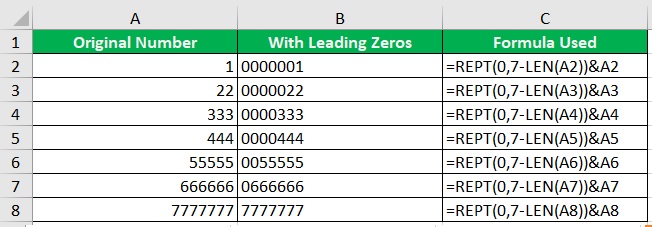
Here’s a visual representation of how the formula works:

The TEXT Function

The TEXT function converts the number to text. But more importantly, we can set the format of the resulting string. We’ll be using this fact to add leading zeros to numbers.

The formula for using the TEXT function is as follows:

=TEXT(number,format)

Where

number – refers to the number or the cell that contains the number

format – sets the format of the resulting string. Make sure to encase it in quotation marks (e.g. “000000”. You can set it the same way you set a custom format. For example, if you want the resulting string to always show a minimum of 7 digits, you set it to “0000000” (if the number has less than seven digits, the formula will add leading zeros).

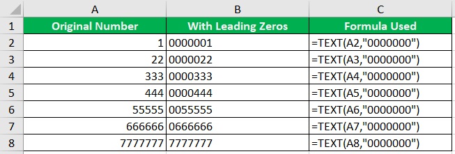
Here’s a visual representation of how the formula works:

Conclusion

And those are the several ways you can make leading zeros appear in Excel.

Some of the methods involve changing cell format, while others involve using formulas.

Which is your preferred method of adding leading zeros?

Let me know in the comments.