How To Separate Addresses in Excel3 Simple Methods


When working with addresses, it is generally ideal to have the information separated into distinct columns, such as home or business number, street address, city, state, and zip code.
This makes it far easier to find, sort, and use this data whenever it is needed.
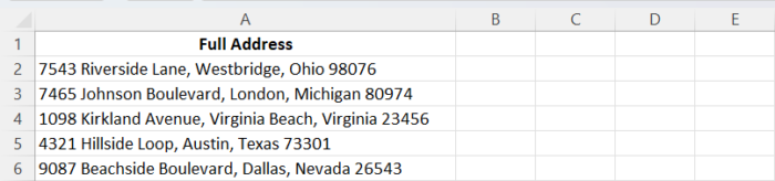
Unfortunately, when it comes to worksheets containing this data, in practice, you will often receive a spreadsheet containing all of this distinct information in only a single column.
This means that if you want to find everyone that lives in a single zip code or city, for example, it may be difficult to reasonably find this information without a considerable degree of extra effort.
Fortunately, however, it is possible to separate addresses into separate columns after they are entered, with each part of the address contained in separate columns.
There are a few ways to do this, and we will show you how you can use each of them.
How To Separate Addresses with Text to Columns
When all of the addresses in your worksheet are delimited with commas, it is easy to use Excel’s “Text to Columns” function to separate the different parts into their own columns.
Because each part of an address may be separated into columns, Excel can use this information to easily separate the different parts of your data into separate columns, and here is how you can use it.
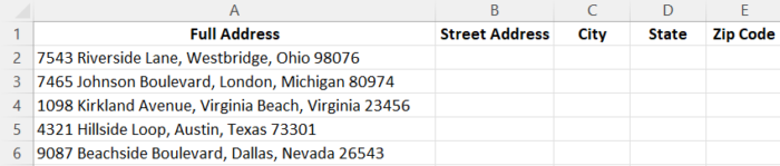
- Place new column headers for each of the new columns where you will place the parts of your addresses, such as a street address, city, state, and zip code.
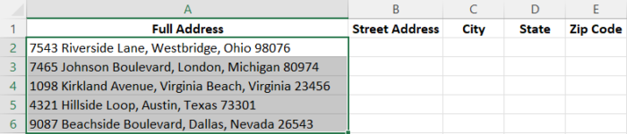
- Select all of the full addresses you wish to split.
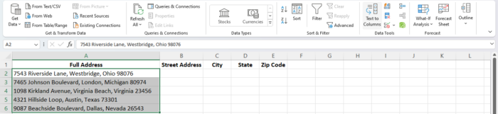
- Navigate to the “Data” tab and under the “Data Tools” group, select the “Text to Columns” icon.
- The “Convert Text to Columns Wizard” will open, displaying the first of three steps. Here ensure that the “Delimited” option is selected and click “Next.”

- For step two within the “Delimiters” group, ensure that the “Comma” option is selected and click “Next.”

- In the final step, enter the “Destination” cell where you want the output to be placed. For example, “$B$2.” Hit “Finish”
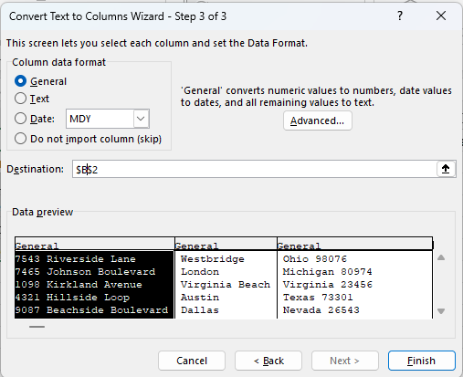
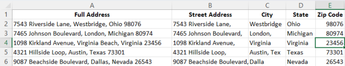
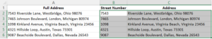
Excel will now split your address into different parts based on how and where the commas were placed. For example, most addresses have a comma between the street address, city, and state, but none before the zip code.
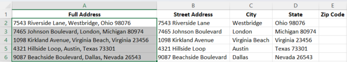
If this is the case, your address will be separated into three sections.
In order to separate the zip code, select the cells in the column where it is located and repeat the earlier steps until you reach step 2 of the “Convert Text to Columns Wizard.”
Earlier, we selected “Comma’ but this time, make sure “Space” is selected.
Complete the remainder of the process, and the Zip Code will now be placed in the appropriate column.
As you can see, this method is extremely easy to use; however, its use is limited to instances in which the same form of delimiter is present between segments of the address information that the “Convert Text to Columns Wizard” can use to determine where breaks should be made.
How To Use the Excel Flash Fill Feature to Separate Addresses
Using the “Text to Columns” is great when your addresses have uniform delimiters, but this will often not be the case in practice.
However, this does not mean you are left without options for easily separating addresses.
In most cases, even if there aren’t uniform delimiters, there is a pattern to how addresses will be listed in spreadsheets.
For example, a hyphen may be used between street address and city, and a comma may be used between city and state.
When there is a pattern like this present in your worksheet, the “Flash Fill” function is a great choice.
This feature allows Excel to extract information from your cells and separate them into distinct columns based on the patterns present in the data.
Simply by providing Excel with a few examples of what you want to do, the program will detect the pattern.
From here, all you need to do is use “Flash Fill” to separate the addresses into the correct columns for you based on the pattern it observed.
Here is how to use “Flash Fill” to separate addresses in your worksheet.
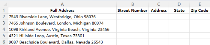
- Start by creating new column headers to receive the different segments of the address data in the columns to the right of the full address.
- Enter the address data manually into the field items in the first two rows. This will provide Excel with the data it needs to detect the pattern present in the data. It will use this to split up the remaining addresses in your worksheet. ( Note that in order to prevent the loss of any leading zeros in the zip code, you should add an apostrophe at the start of any zip code.)
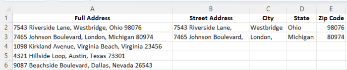
- Now select the first blank cell in the following row.
- Use the keyboard shortcut (CTRL + E) or the “Flash Fill” button found under the “Data” tab within the “Data Tools” group to have “Flash Fill” input the address data into each of the cells in the row.
- Now use “Tab” to move to the next column and repeat the previous step to input data into the cells within the column.
- Now you can repeat the previous two steps as many times as you need to separate all of the addresses in your worksheet.
How To Separate Addresses with Excel Formulas
One of the best aspects of using Excel for organizing and storing data is its ability to use functions in order to filter and perform operations on data.
You can also use formulas as a way to separate each of the parts of addresses as well.
So even if none of the previous two methods worked for you, it is still possible to separate your addresses using an Excel formula to do the job.
Though it may not be the easiest method, it is definitely the most flexible, and you can customize the method we will show you to separate whatever style of address is present in your worksheet. Here is how.
- Start by selecting the header of the column in which your addresses are located and then press the “Shift” key on your keyboard while clicking on the column header to the column’s right. Select the “Home” tab and select the arrow icon next to “Insert.” Click on the “Insert Sheet Columns” in order to place an additional two blank columns to the right of the addresses.
- Select the first cell in the column to the right of your addresses. Assuming your worksheet has labels at the top of every column, you would select cell B2, which would be to the right of cell A2.

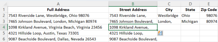
3. Next, click into the formula bar, type the formula =LEFT(A2,FIND(” “,A2,1)), and press Enter. Excel will scan the text in cell A2 from left to right to locate the first space, which typically appears right after the building number in an address. It will then extract all the characters up to that space and return the result in cell B2.
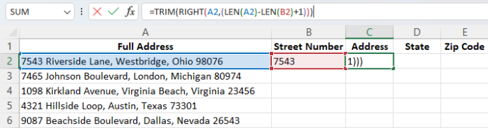
4. Now select cell C2 and enter =TRIM(RIGHT(A2,(LEN(A2)-LEN(B2)+1))). Once you run this formula, Excel will take data in the address with the exception of the building number and eliminate the empty space at the start before displaying it.
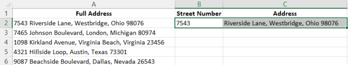
5. Now select both B2 and C2 and hover your cursor over the lower right-hand corner of these cells. When the cursor changes into a “+” icon, drag it over the below cells to apply the formula to these cells. Excel will automatically alter the cell references for the appropriate rows.
Setting up formulas to separate addresses can take a little bit of time, but the effort is well worth it as you may need to change “full address” cells down the line.
With this method, once you understand the formula, it is easy to adjust parameters to suit your needs.
Conclusion
Now you have seen how to separate the different parts of an address into separate columns in Excel.
This includes how to separate addresses with delimiters through “Text to Columns” as well as addresses with a pattern to how they are listed in a spreadsheet.
Finally, you have seen how to use an Excel formula to separate the addresses as well.
No matter which method you choose, all of these are flexible and effective ways to separate addresses.
Now you can see that it is easy to separate your addresses in Excel no matter which method you feel comfortable with.