Apply Horizontal Filter in ExcelLearn how to filter horizontal data in Excel

When you’re working with a large dataset, it can be impractical to look at it entirely if you only want certain data.

For example, let’s say you’re working with a worksheet that contains data regarding the monthly sales of your sales personnel.

Now, you only want to take a look at the monthly sales performance of a particular sales agent.

What do you? Scour the entire worksheet for such data? That’s inefficient.

The better thing to do here is to filter your data.

Fortunately, Excel has a Filter feature.

With just the click of a button, you can filter your data.

But the thing with this Filter feature is that it only applies vertical filters.

As such, it works best if the data you’re working on is oriented vertically.

But what if isn’t? What if the data is oriented horizontally? Here’s an example:

When I try to apply filters using Excel’s Filter feature, it still applies to vertical filters:

So if you want to apply horizontal filters, the Filter feature won’t be able to help you. But don’t lose hope yet. Excel has other functions and features that you can to filter horizontal data.

In this article, we’ll be discussing how to apply horizontal filters in Excel.

By the end of the article, you should be able to consistently and reliably filter horizontal data anytime you need to.

Let’s get started.

Use the FILTER Function to Apply Horizontal Filters in Excel

In the recent versions of Excel (Office 365 and Excel 2021), dynamic arrays were added. Along with this addition came the FILTER function.

Not to be confused with the Filter feature, the FILTER function returns a dynamic array that filters the referenced array depending on the criteria set by the user.

This resulting dynamic array will follow the shape of the referenced array. Thus, if the referenced array is oriented horizontally, the resulting array will also be oriented horizontally.

We will be using this fact to our advantage (such as by applying horizontal filters).

One of the more noticeable differences between the Filter feature and the FILTER function is that the former can be accessed via the Filter button on the Data tab, while the latter can be accessed via a formula. Speaking of, here’s the formula for using the FILTER function:

=FILTER(array,criteria,if_empty)

Where

array – refers to the array or range of cells from which you want to filter data from

criteria – this specifies by which criteria the FILTER function will filter data

if_empty – this is the value that appears when the FILTER function does not return any data based on the other parameters.

This parameter is optional and has a default value of “#CALC!”. Make sure to enclose the value in parentheses (e.g.  “NO DATA”, “NULL”)

How to Apply Horizontal Filters

We’ll be using the following dataset for illustration:

Suppose you want to apply horizontal filters to this data so that you can see the monthly sales data of a specific Sales Agent. To do so, you’ll be using the FILTER function.

Before that though, you set the worksheet as follows:

• Select an empty. Make sure that this cell has enough adjacent empty cells to the right and the bottom. In our illustration, this will be cell B8.
• In the selected cell, enter the formula for the FILTER function. In our illustration, the formula will be =FILTER(B1:M3,B2:M2=B6,”NO DATA”). array is set to B1:M3 because this is the range of cells that contains the data that we want to filter. criteria is set to B2:M2=B6 because we want to filter by Sales Agent and cell B6 is where we enter the filtered for the specified Sales Agent. if_empty is set to “NO DATA” so that the resulting array will show NO DATA if the FILTER function returns an empty array.

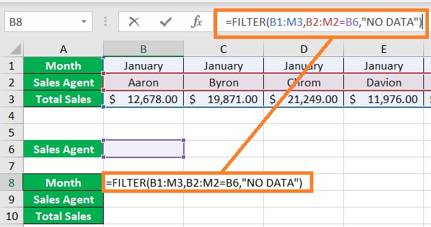
• Press the Enter key. The formula should return a NO DATA value for now. This is because the filter criteria are not set yet.

• In cell B6, enter Chrom so that the FILTER function returns the monthly sales data of Sales Agent Chrom.

And there you have it. You have successfully applied horizontal filters by using the FILTER function.

Create Custom Views to Filter Horizontal Data in Excel

If you’re using a version of Excel that doesn’t have dynamic arrays, then using the FILTER function is not an option for you.

But there’s a workaround for this: creating custom views.

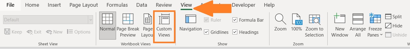
To create custom views, you’ll have to open the View tab.

On the left side of the ribbon, you should see the Custom Views button.

We’ll be using this feature to filter data that is oriented horizontally.

How to Filter Data Horizontally

Suppose you’re working with the following dataset:

• Open the View tab. Click the Custom Views button.

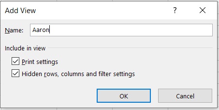
• This will open the Custom Views window. In this window, click add.

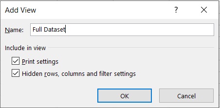
• You’ll be asked to name the new view. Since you’re currently looking at the entire dataset (unfiltered data), you may set the name to “Full Dataset”. Click the OK button after doing so.

• You’ll now create the first filtered view, which will be the monthly sales data of Sales Agent Aaron. Hide the columns that do not contain Aaron as the Sales Agent.

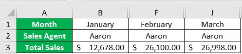
• Create a custom view for Aaron’s monthly sales data.

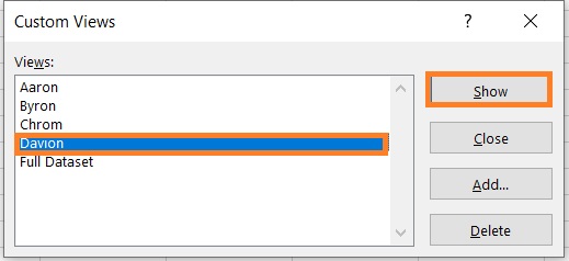
• Do the same steps for each Sales Agent. By the end, your Custom Views window will look like this:

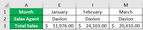
• To show filtered data, just select the custom view that you want to see, then click the Show button. For example, we want to see the monthly sales data of Sales Agent Davion.

You have successfully filtered data horizontally by creating custom views.

Transpose and Filter Horizontal Data in Excel

If you find creating custom views tedious, then there’s another option for you.

Technically, you won’t be applying horizontal filters with this method. But you’ll still be filtering the same data. To do so, you’ll be transposing data. What this does is swap the columns and rows.

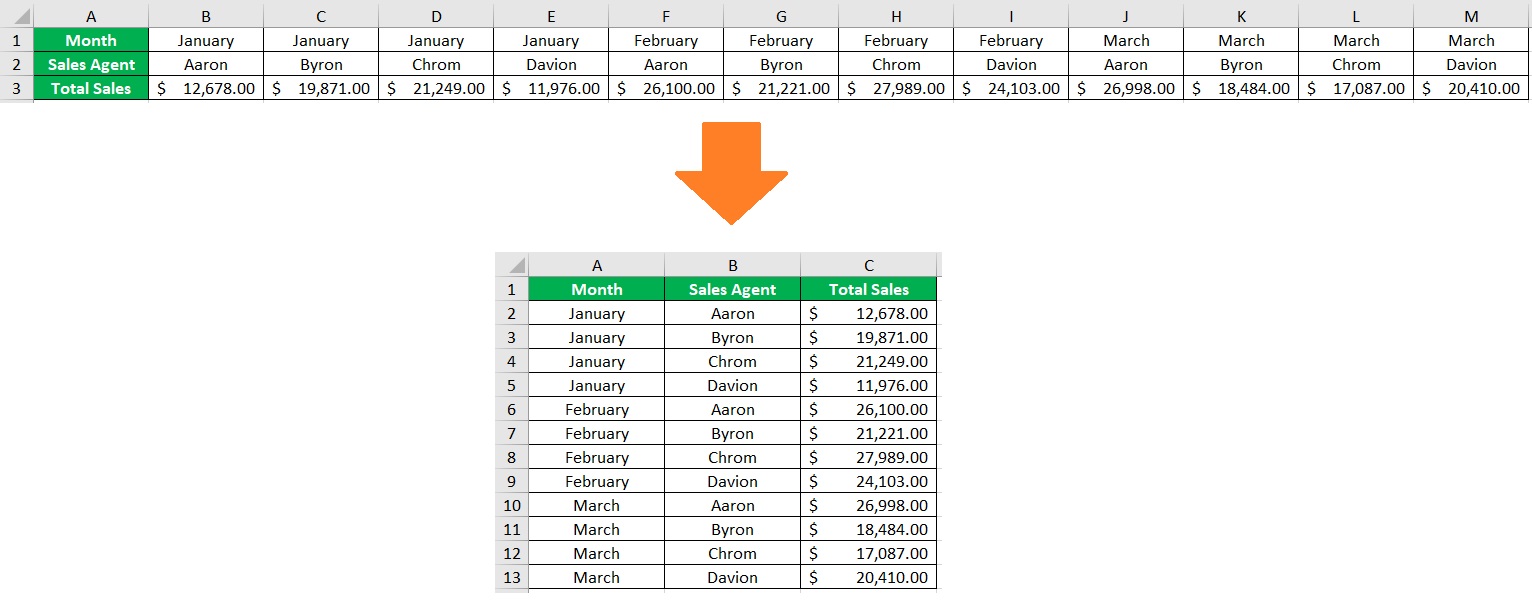
With the data being transposed, you can then use Excel’s Filter feature. Here are the steps to do so.

How to Filter Horizontal Data

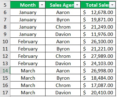
Suppose you’re working with this dataset:

• Select the entire dataset. Press the keyboard shortcut Ctrl + C to copy the dataset.

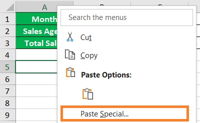
• Select an empty cell (in our illustration, this will be cell A5). Right-click on the cell. This will present you with a list of options. Select Paste Special from among them.

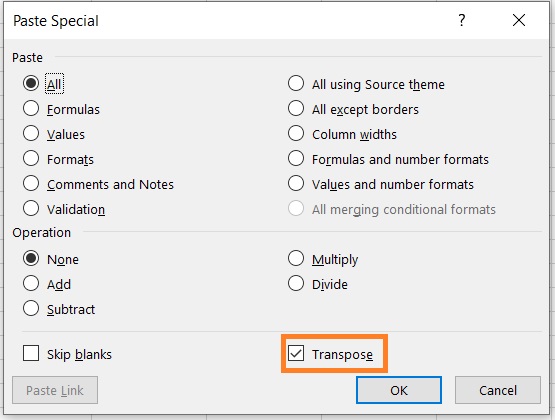
• This will open the Paste Special menu. Tick the box next to Transpose and then click the OK button.

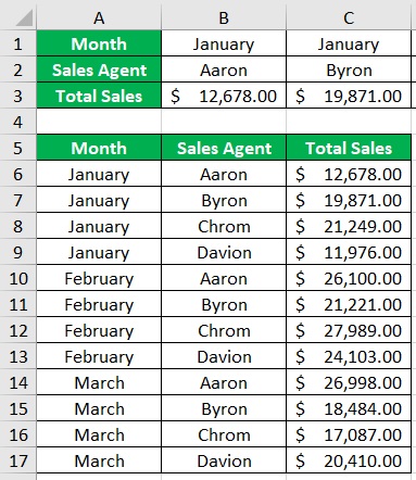
• You have successfully transposed the dataset.

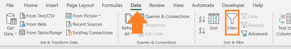
• Select the transposed dataset. Apply filters by opening the View tab and clicking on the Filter button.

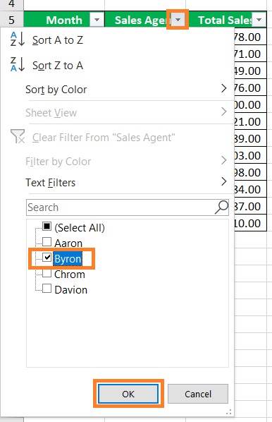
• Suppose you want to look at the monthly sales data of Sales Agent Byron. Just click on the filter button next to the Sale Agent column header. Then, make sure that only the box next to “Byron” is ticked.

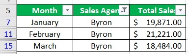
• You have successfully filtered the dataset.

Conclusion

And those are the different methods you can follow to filter data that is oriented horizontally.

You should now be able to filter horizontal data anytime you need to.