Flip Data (as Well as Charts) in ExcelLearn how to flip data and charts vertically and horizontally in Excel


With how often you work with tables or structured datasets (those that are arranged in columns and/or rows) in Excel, you would think that flipping data would be a default feature.
I hate to break it to you, but currently, Excel doesn’t have a one-click feature for that yet.
Now, flipping sorted data isn’t that much of an issue.
You can easily use Excel’s sort feature to change the sort order for sorted data (change it to ascending or descending order).
The issue comes with unsorted data.
If you use Excel’s sort feature to reverse the order of unsorted data, you will most probably jumble the original order of the data.
So, how are you to flip or reverse the order of unsorted data in Excel?
Is there no other way than to manually flip the order?
I can’t imagine having to flip the order of a hundred rows and columns of data, much more a thousand. Surely there’s another way, right?
Well, turns out that there’s just more than one way to flip data in Excel, be it vertically or horizontally.
And in this article, we’ll be discussing those ways. And as a bonus, I’ll be showing you how to flip charts in Excel.
Are you raring to flip data in Exel?
Let’s get started then!
Use Helper Column or Row to Flip Data in Excel
For the first method, we’ll be employing the services of a helper column to flip data vertically, and a helper row to flip data horizontally.
A helper column or row is simply an extra column/row where we put a sequence of numbers.
This will define the original order of the dataset.
With it, we can flip the dataset without jumbling the order (we only reverse the original order). It’ll be much easier to explain with illustrations.
How to Flip Data Vertically
Suppose we have this dataset:
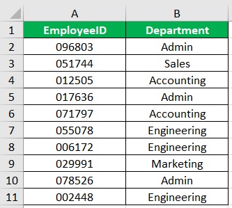
We want to flip this dataset (i.e. reverse the order). To do so, we’ll be using a helper column.
Here are the steps:
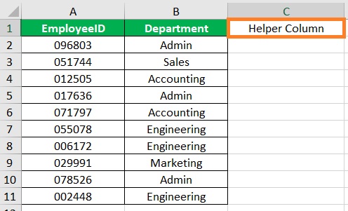
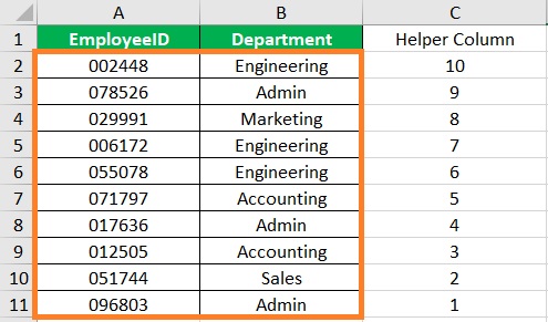
- Make sure that the column that is adjacent to the rightmost column of the dataset is empty. If it isn’t, insert a new column. This will be our helper column. Let’s give it the column header “Helper Column”.
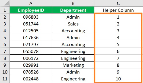
- Next, fill in this column with a sequence of numbers (e.g. 1, 2, 3…). Do it until the next empty row. (TIP: You can use the SEQUENCE function to quickly fill in the column. Just make sure to copy the resulting array and paste its values).
- Now that we have our helper column, we can safely use the sort feature to flip the dataset. To do so, select the helper column. Then, open the Data tab. You should see a Sort & Filter section along the ribbon.
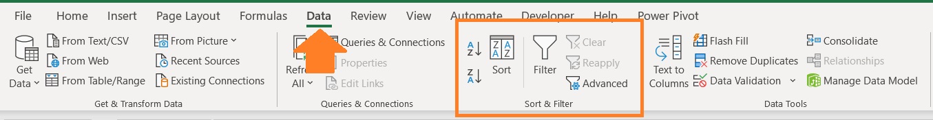
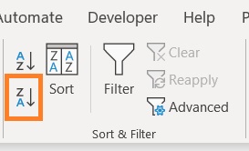
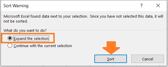
- In the Sort & Filter section, click the Sort Z to A button (shown in the image below). A Sort Warning should pop up. Select the “Expand the Selection” option then click the Sort button.
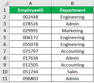
- We have successfully vertically flipped the dataset.
- We can now delete the helper column as it has already done its job.
How to Flip Data Horizontally
Suppose the dataset was arranged horizontally:

We want to flip this dataset horizontally. To do so, we’ll be using a helper row. Here are the steps:
- Make sure that the row that is directly below the bottom row of the dataset is empty. If it isn’t, insert a new row. This will be our helper row. Let’s give it the row header “Helper Row”.

- Next, fill in this row with a sequence of numbers (e.g. 1, 2, 3…). Do it until the next empty column. (TIP: You can use the SEQUENCE function to quickly fill in the column. Just make sure to copy the resulting array and paste its values).

- Now that we have our helper row, we can safely use the sort feature to flip the dataset. To do so, select the dataset (including the helper row). Then, open the Data tab. You should see a Sort & Filter section along the ribbon.
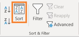
- In the Sort & Filter section, click the Sort button (shown in the image below). This will open the Sort dialog box.
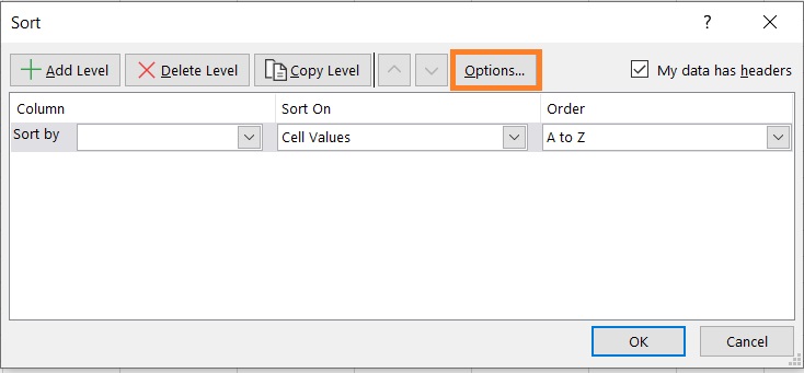
- In the Sort dialog box, click the Options button.
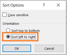
- A Sort Options will pop up. Select the “Sort left to right” option, and then click the OK button. This will allow us to horizontally flip the dataset.
- Back to the Sort dialog box. In the textbox after “Sort by”, select the row number of the helper row (in our illustration, it is Row 3).
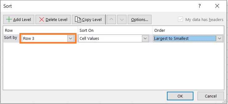
- In the textbox below “Sort On”, select Cell Values.
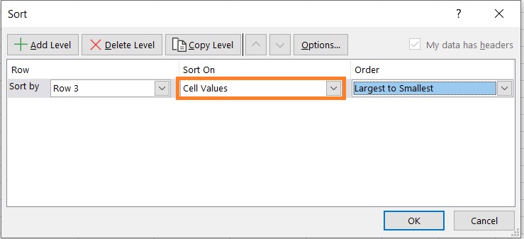
- In the textbox below Order, select Largest to Smallest. Then, click the OK button.
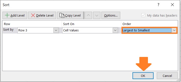
- We have successfully horizontally flipped the dataset.

- We can now delete the helper row as it has already done its job.

Use Formula to Flip Data in Excel
For the next method, we’ll be using a formula to flip the data vertically or horizontally.
This formula incorporates the INDEX, ROWS, and COLUMNS functions.
Let me show you the formulas first before I explain what they do.
To flip data vertically, the formula to use is as follows:
=INDEX(range,ROWS(range))
Where
range – refers to the range of cells that contains the data that you want to flip
To flip data horizontally, the formula to use is as follows:
=INDEX(range,ROWS(range),COLUMNS(range))
Where
range – refers to the range of cells that contains the data that you want to flip
Some information about the formulas:
- The range for the INDEX function should be an absolute reference. This means that there should be a $ symbol before the column letters and row numbers. This is so that when we copy the formula to the other rows or columns, the INDEX array isn’t changed.
- For the range for the ROWS and COLUMNS functions, we only need to make an absolute reference to the end of the range. This is so that the number of rows or columns changes as we copy the formula to the other rows or columns.
- Since we’re using a formula to flip data, the result will be dynamic. This means that if there are any changes to the referenced range of cells, the result will automatically update.
- Copy and paste the result as values to make it (the result) static. This will allow us to delete the original data without affecting the result.
How to Flip Data Vertically
Suppose we have this dataset:
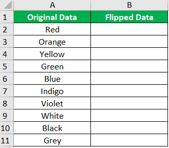
In the flipped data column, we aim to fill it in with the flipped order of the original data.
To do so, we’ll be using a formula that incorporates the INDEX and ROWS functions.
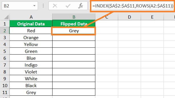
- Select the cell adjacent to the first cell of the dataset (other than the column header). In our illustration, this will be cell B2.
- In the selected cell, enter the formula for flipping data vertically. Makes sure that the INDEX range is an absolute reference. For the ROWS range, only make an absolute reference to the end of the range. In our illustration, the formula will be =INDEX($A$2:$A$11,ROWS(A2:$A$11)).
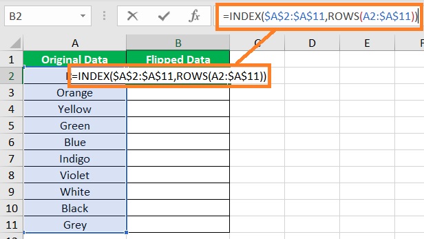
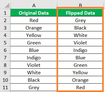
- Press the Enter key to execute the formula. Then, copy the formula to the rest of the column (until the next empty row).
- We have successfully flipped the data vertically.
How to Flip Data Horizontally
Now let’s try the horizontal flip version of the formula on this dataset:

In the flipped data row, we aim to fill it in with the flipped order of the original data.
To do so, we’ll be using a formula that incorporates the INDEX, ROWS, and COLUMNS functions.
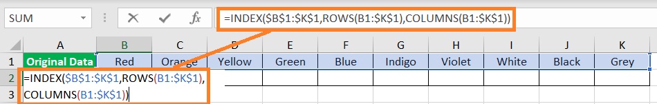
- Select the cell below the first cell of the dataset (other than the row header). In our illustration, this will be cell B2.
- In the selected cell, enter the formula for flipping data horizontally. Makes sure that the INDEX range is an absolute reference. For the ROWS range, only make an absolute reference to the end of the range. The same goes for the COLUMNS range. In our illustration, the formula will be =INDEX($B$1:$K$1,ROWS(B1:$K$1),COLUMNS(B1:$K$1)).
- Press the Enter key to execute the formula. Then, copy the formula to the rest of the column (until the next empty row).
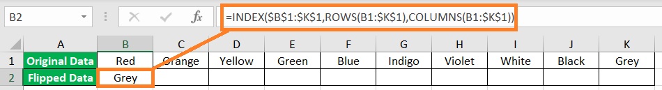
- We have successfully flipped the data horizontally.

Use VBA to Flip Data in Excel
If you know how to use the VBA feature in Excel, then here are the VBA codes you can use to flip data in Excel:
Flip Data Vertically (Flip Columns) in Excel Using VBA
The VBA code that you’ll be using to flip data vertically (flip columns) in Excel is as follows:
Sub FlipColumn()

Dim Rng As Range

Dim WorkRng As Range

Dim Arr As Variant

Dim i As Integer, j As Integer, k As Integer

On Error Resume Next

xTitleId = "Flip columns"

Set WorkRng = Application.Selection

Set WorkRng = Application.InputBox("Range", xTitleId, WorkRng.Address, Type:=8)

Arr = WorkRng.Formula

Application.ScreenUpdating = False

Application.Calculation = xlCalculationManual

For j = 1 To UBound(Arr, 2)

k = UBound(Arr, 1)

For i = 1 To UBound(Arr, 1) / 2

xTemp = Arr(i, j)

Arr(i, j) = Arr(k, j)

Arr(k, j) = xTemp

k = k - 1

Next

Next

WorkRng.Formula = Arr

Application.ScreenUpdating = True

Application.Calculation = xlCalculationAutomatic

End Sub
Flip Data Horizontally (Flip Rows) in Excel Using VBA
The VBA code that you’ll be using to flip data horizontally(flip rows) in Excel is as follows:
Sub FlipRows()

Dim Rng As Range

Dim WorkRng As Range

Dim Arr As Variant

Dim i As Integer, j As Integer, k As Integer

On Error Resume Next

xTitleId = "Flip Rows"

Set WorkRng = Application.Selection

Set WorkRng = Application.InputBox("Range", xTitleId, WorkRng.Address, Type:=8)

Arr = WorkRng.Formula

Application.ScreenUpdating = False

Application.Calculation = xlCalculationManual

For i = 1 To UBound(Arr, 1)

k = UBound(Arr, 2)

For j = 1 To UBound(Arr, 2) / 2

xTemp = Arr(i, j)

Arr(i, j) = Arr(i, k)

Arr(i, k) = xTemp

k = k - 1

Next

Next

WorkRng.Formula = Arr

Application.ScreenUpdating = True

Application.Calculation = xlCalculationAutomatic

End Sub
Flip Charts in Excel Vertically or Horizontally
Flipping charts in Excel is fairly quick and easy compared to flipping datasets.
It’s only a matter of reversing the order of the x-axis (to flip the chart horizontally) or the y-axis (to flip the chart vertically.
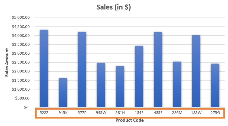
Suppose we have this chart here:
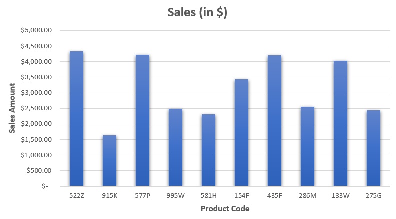
Let’s try flipping this chart vertically and horizontally.
How to Flip Chart Vertically
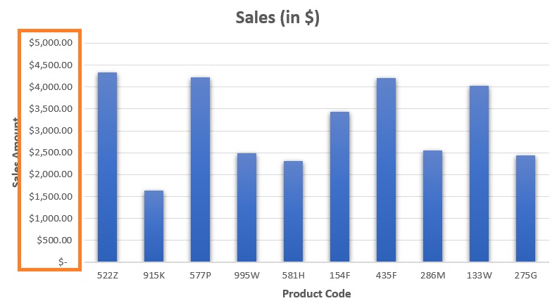
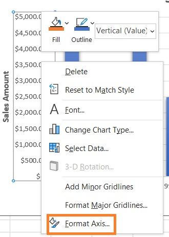
- First, select the chart. Then, right-click on any of its y-axis labels.
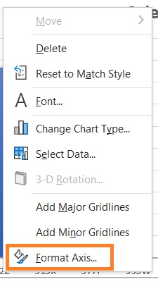
- From the options that appear after right-clicking, select “Format Axis”.
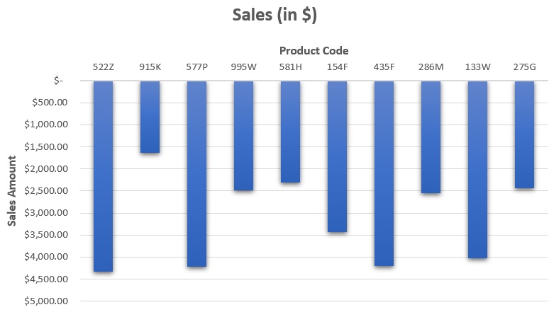
- This will open the Format Axis sidebar. Under Axis Options, we should see an option to set the Values in reverse order. Tick the box before it (make sure that it is checked).
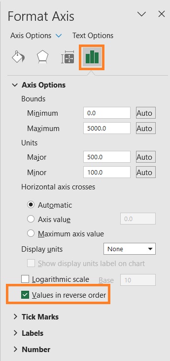
- We have successfully flipped the chart vertically.
How to Flip Chart Vertically
- First, select the chart. Then, right-click on any of its x-axis labels.
- From the options that appear after right-clicking, select “Format Axis”.
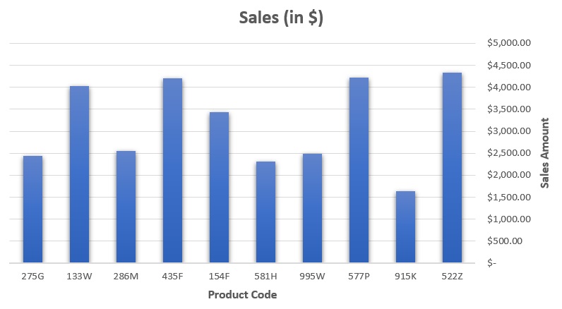
- This will open the Format Axis sidebar. Under Axis Options, we should see an option to set the Categories (or Values, depending on the data type) in reverse order. Tick the box before it (make sure that it is checked).

- We have successfully flipped the chart horizontally.
Conclusion
And those are the different we can flip data in Excel.
It may not be as simple as a one-click operation, but it certainly beats manually flipping a whole dataset.
We also discussed how to flip Excel charts in this article.
Now go and have fun flipping things in Excel!