Find Duplicates in ExcelLearn how to find duplicates in Excel (as well as remove them)


You may sometimes work on a dataset that has duplicates. It could be intentional. That’s fine.
What isn’t is if it’s unintentional. In such a case, you have to identify these duplicates.
Then, you’ll have to remove them since they weren’t supposed to be there in the first place.
Doing this manually is fine if you’re only working with a small dataset.
But what if you’re working with a large dataset?
I’m talking about a thousand or more entries!
Seem very time-consuming, isn’t it?
Not to mention that it’s prone to human error.
Thankfully, Excel has features that can help you find and identify duplicates within a dataset.
It even has a dedicated button for removing duplicate entries. In this article, you’ll be learning how to use these Excel features.
By learning how to use them, you’ll be able to find and identify (even remove) duplicates in Excel whenever you have to.
Let’s get started.
Use Conditional Formatting to Find Duplicates in Excel
The first feature that you’ll be using to find duplicates is Excel’s Conditional Formatting.
This nifty feature can be accessed via the Home tab.
Located somewhere in the middle right section of the ribbon is the button to access Conditional Formatting:

Clicking on this button will present you with the following options:

Among these options is the Highlight Cells Rules option, which you can use to find and highlight duplicates within a dataset. Here are the steps to do so.
How to Find and Highlight Duplicates
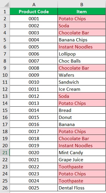
Suppose that you’re working with the following dataset:
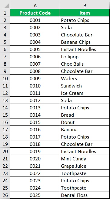
Each item is assigned a unique product code. An item should only be assigned one product code.
However, when you examine the dataset, you find that some items are assigned several product codes.
Your goal here is to identify the items that have duplicate entries within the dataset.
This way, you can highlight which items have been assigned several product codes.
To do so, you’ll be using Excel’s conditional formatting.
- Select the cells that you want to check duplicates for. If you want to check the whole sheet, press the keyboard shortcut Ctrl + A to select all cells within the sheet.
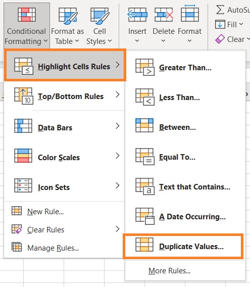
- Open the Home tab. Somewhere in the middle right section of the ribbon, you should find the Conditional Formatting button. Click on it.
- You’ll be presented with several options. Among these options is the Highlight Cells Rules option. Select it. Then from the following options, select Duplicate Values.
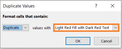
- A Duplicate Values dialog box will open. It will contain two dropdown boxes. The first dropdown box contains the options “Duplicate” and “Unique”. Since your goal is to find duplicates, choose the “Duplicate” option.

- The other dropdown box contains options on how the cells that contain duplicates will be highlighted. For now, choose the “Light Red Fill with Dark Red Text” option.
- Click the OK button.
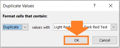
- You should now find that cells containing duplicates are now highlighted.
Use the COUNTIF Function to Find Duplicates in Excel
Another Excel feature you can use to find duplicates in a dataset is the COUNTIF function.
The COUNTIF function is a bit more versatile than Conditional Formatting in that you can use it to find duplicate values within a column, or find duplicate rows within a dataset.
The formula for using the COUNTIF function to identify duplicate values within a column is as follows:
=COUNTIF(column,value)>1
Where
column – refers to the column from which you’ll be finding duplicates of value in
value – refers to the value (or cell reference) that you’re checking for duplicates
How to Find Duplicate Values Within a Column
Suppose that you’re working with the following dataset:
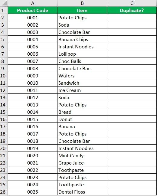
Each item is assigned a unique product code. An item should only be assigned one product code.
However, when you examine the dataset, you find that some items are assigned several product codes.
Your goal here is to identify the items that have duplicate entries within the dataset. This way, you’ll know which items have been assigned several product codes.
To do so, you’ll be using the COUNTIF function.
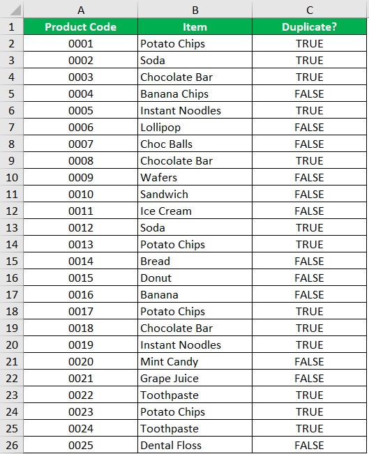
- Select an empty cell. Ideally, it should be adjacent to the cell that you’ll be checking for duplicates. For our illustration, this will be cell C2.
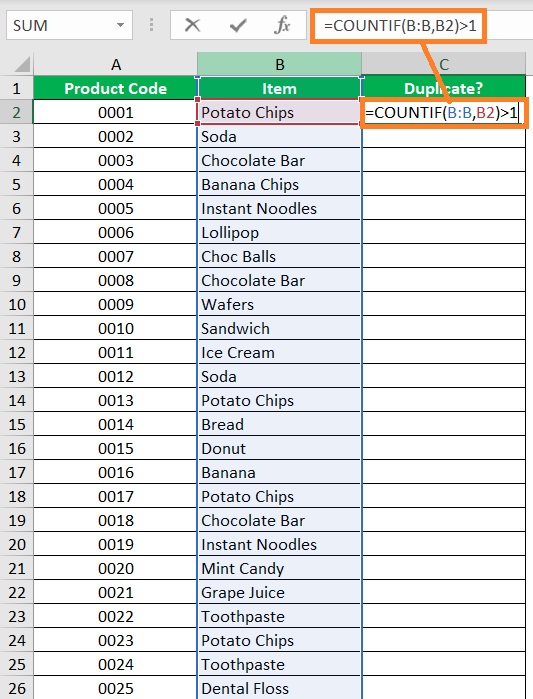
- In the selected cell, enter the formula for using the COUNTIF function to identify duplicate values within a column. For our illustration, the formula will be =COUNTIF(B:B,B2)>1.
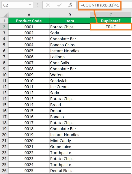
- Press the Enter The COUNTIF function will return with either of these two values: TRUE or FALSE. It will return a TRUE value if the reference cell has duplicates within the column. It will return a FALSE value if the reference cell is a unique value.
- Copy the formula to the rest of the column (until the next empty row).
You can also nest the COUNTIF formula within an IF formula to change the TRUE and FALSE values into something more significant (e.g. Duplicate and Unique). Here’s an example formula:
Use the formula `=IF(COUNTIF(B:B,B2)>1,”DUPLICATE”,”UNIQUE”)` to quickly identify whether a value in cell B2 appears more than once in column B. If it does, the formula returns “DUPLICATE”; if it appears only once, it returns “UNIQUE,” helping you efficiently spot repeated entries in your data.

Use the COUNTIFS Function to Find Duplicate Rows in Excel
A variation of the COUNTIF function is the COUNTIFS function.
This function can be to find duplicate rows or duplicate values within several columns.
The formula for using the COUNTIFS function is similar to the COUNTIF function.
It’s like nesting a ton of countif functions without actually nesting formulas:
=COUNTIFS(column1,value1,column2,value2….)>1
Where
column – refers to the column from which you’ll be finding duplicates of value in
value – refers to the value (or cell reference) that you’re checking for duplicates
To make it easier to identify duplicate rows, let’s nest the COUNTIFS formula within an IF formula:
=IF(COUNTIFS(column1,value1,column2,value2)>1,“DUPLICATE ROW”,“”)
This way, the COUNTIFS function will show a “DUPLICATE ROW” value if the row has duplicates, and will return a blank if it’s unique.
How to Find Duplicate Rows
Suppose that you’re working with the following dataset:
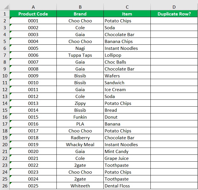
This time, aside from checking the item for duplicates, you have to check its brand too.
The same items but different brands can be assigned different product codes.
However, items that are of the same brands should still be assigned just one product code.
This means that you’ll be checking duplicates within several columns (or checking for duplicate rows).
To do so, you’ll be using the COUNTIFS function.
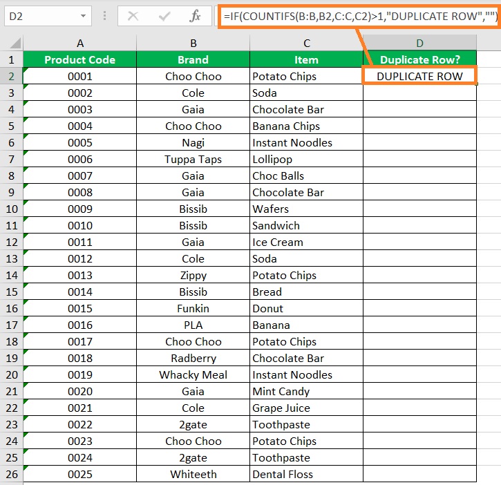
- Select an empty cell. Ideally, it should be adjacent to the cells that you’ll be checking for duplicates. For our illustration, this will be cell D2.
- In the selected cell, enter the formula for using the COUNTIFS function to identify duplicate values within several columns. For our illustration, the formula will be =IF(COUNTIFS(B:B,B2,C:C,C2)>1,”DUPLICATE ROW”,””).

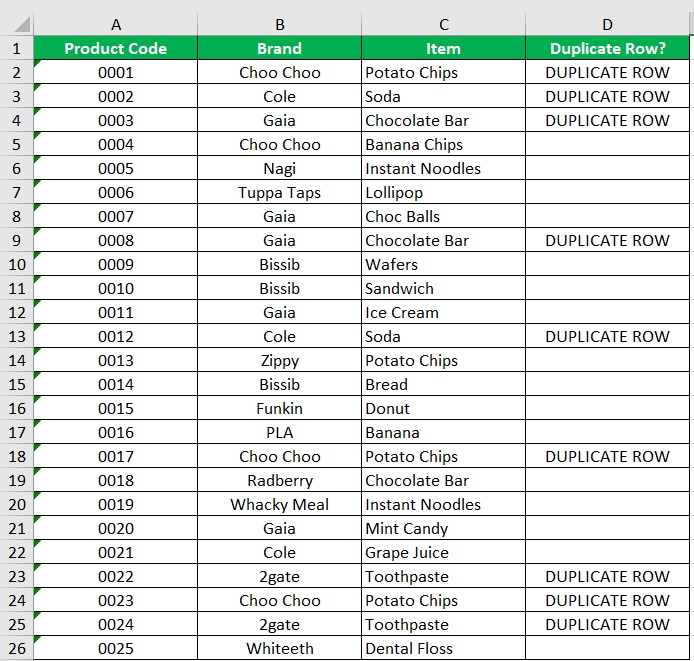
- Press the Enter The COUNTIFS function will return with return a “DUPLICATE ROW” value if there are duplicates. Otherwise, it will return a blank value.
- Copy the formula to the rest of the column (until the next empty row).
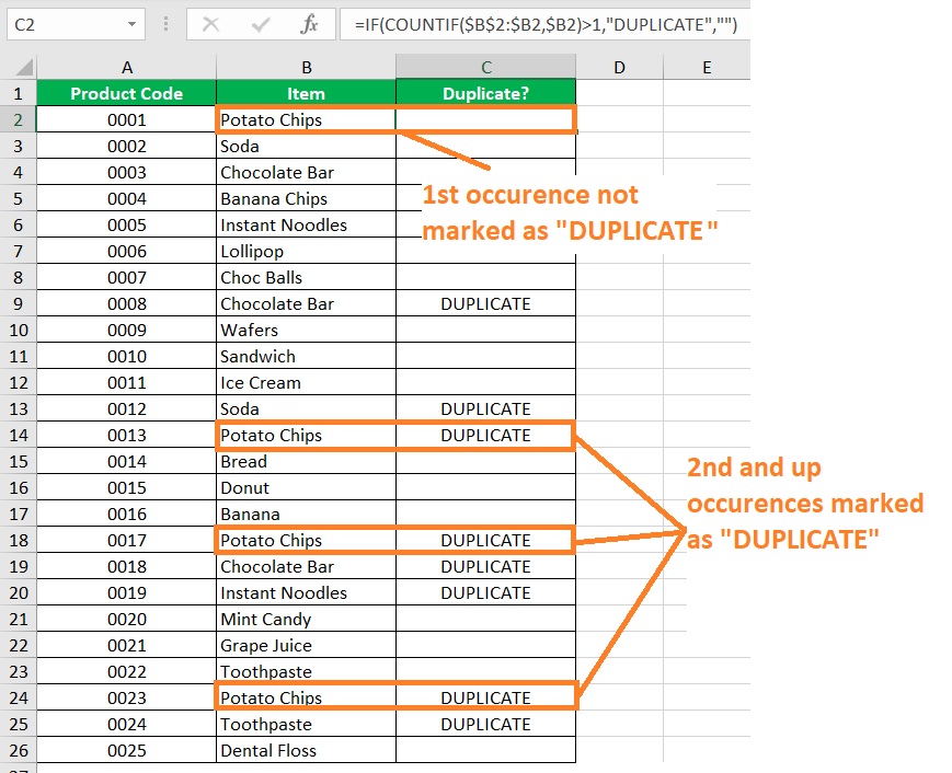
Marking only the 2nd Occurrence of A Duplicate (Using COUNTIF and COUNTIFS)
The above COUNTIF and COUNTIFS formulae will mark all duplicate values as duplicates, which could be tricky if you want to remove all duplicates but retain the original.
In such a case, you want to mark the first instance to be a unique value.
You also want to mark the rest of the instances as duplicates.
To do so, you’ll have to modify your COUNTIF formula.
For example, let’s modify our COUNTIF formula above. We’ll be using the following formula instead:
=IF(COUNTIF($B$2:$B2,$B2)>1,”DUPLICATE”,””)
This way, a duplicate will only be marked as “DUPLICATE” if it’s the 2nd or up occurrence.
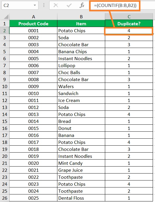
Count Instances of Each Duplicate (with the COUNTIF Function)
The above uses of the COUNTIF function are to identify the duplicates within a selection.
However, you can also use it to count the instances of each duplicate.
To do so, you only need to remove the >1 argument from the formula.
For example, the formula will only be =COUNTIF(B:B,B2).
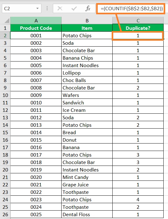
If you want to identify whether it’s the 1st, 2nd, 3rd, or so occurrence, you can also modify the COUNTIF formula.
For example, we’ll be using the formula =(COUNTIF($B$2:$B2,$B2)).
Easily Remove Duplicates Using the Remove Duplicates Button
If you want to go straight to removing duplicates within a dataset, there’s a shortcut where you don’t have to do any of the above procedures.
And you’ll be doing it by using the Remove Duplicates button.
To access this button, you need to open the Data tab. In the middle section of the ribbon, you should find the Remove Duplicates button.

You can use it to remove duplicates from a single column or multiple columns. You can also use it to remove duplicate rows.
For example, I want to remove duplicates from Column B. I’ll first select the column and then click on the Remove Duplicates button.
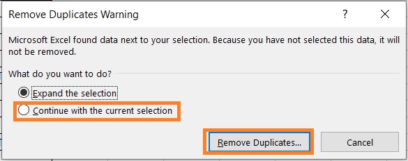
This warning message will pop-up:
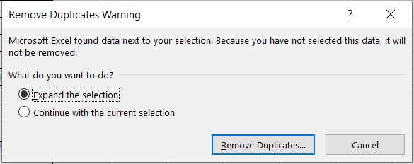
This only pops up if we select a single column while the sheet has other filled columns. Since I want to remove duplicates from Column B, I’ll choose the “Continue with the current selection” option. I will then click the Remove Duplicates button.
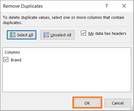
This will open the Remove Duplicates dialog box. All you need to do here is click the OK button.
Excel will inform me how many duplicates it removed and how many unique values remain.
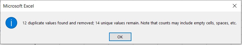
And the duplicates within the column should be removed now.
Conclusion
And those are the ways to find duplicates in Excel, as well as how to easily remove them.
I hope that you’ll be able to use your learnings here in your future endeavors.