Find a Dataset’s Range in ExcelHere are easy ways to calculate a dataset's range in Excel

Last Updated: December 21, 2022

Written By:
Patrick Louie

Reviewed By:
FundsNet Staff

In Excel, you can perform tons of statistical calculations with the help of formulae and Excel functions.

You can calculate the mean, median, standard deviation, etc.

Among these statistical variables is a dataset’s range.

Calculating a dataset’s range is pretty simple.

You only need to subtract its minimum or smallest value from its maximum or largest value.

If we were to present it in formula form, it will look like this:

Range = Maximum Value – Minimum Value

For example, let’s say that you have the following dataset: (1, 4, 5, 2, 3, 8).

This dataset’s minimum value is 1 while its maximum value is 8.

To calculate the range, we simply need to calculate the difference between these two values:

Range = Maximum Value – Minimum Value

= 8 – 1

= 7

As per our calculation, the dataset’s range is 7.

Unfortunately, there is no dedicated Excel function for calculating a dataset’s range.

However, that doesn’t mean that we can’t calculate a dataset’s range in Excel.

We only need to get creative with it. Besides, you only need to perform a simple mathematical calculation to determine a dataset’s range.

What we need to do is to use Excel features to find the dataset’s minimum and maximum values.

In this article, we’ll be learning how to calculate a dataset’s range in Excel.

While it may not be as intuitive as calculating standard deviation or mean, it’s still easy to follow so you shouldn’t have a hard time with it. Let’s get started!

What is Range? What are its Real World Applications?

The range is a numerical representation of a dataset’s or a series’ spread in values.

Simply put, it is the difference between a dataset’s or series’ minimum and maximum values.

Finding a dataset’s range has many applications in the real world.

For example, you want to know the difference between a company’s highest and lowest salaries.

You’re doing so because you want to find out if the company values its lower-level employees just as much as its executive-level employees.

And do to so, you only have to find the range of the company’s salaries.

For another example, let’s say that you’re managing a grassroots basketball team.

You want to determine their consistency in scoring. So you make a list of their scores from recent games.

From here, you can calculate the range to determine their consistency in scoring.

The higher the range, the less consistent they are.

On the other hand, if the range is low, it could indicate that the team is consistent in scoring.

Use the MIN and MAX Functions to Calculate a Dataset’s Range in Excel

For the first method, we will be using the combination of the MIN and MAX functions. These two functions find the dataset’s minimum and maximum values respectively.

The MIN Function

The MIN function finds the smallest or minimum value in a range of values.

The formula to calculate it is as follows:

=MIN(range of values)

Here, the range of values could refer to a set of numbers or a range of cells. For example, let’s say that you want to find the minimum value from this dataset: (8, 7, 1, 0, 2, 3, 3, 4).

The formula will then be:

=MIN(8,7,1,0,2,3,3,4)

If you want to calculate the minimum value contained in cells A2 to A11, the formula will then be:

=MIN(A2:A11)

The MAX Function

The MAX function finds the largest or maximum value in a range of values. The formula to calculate it is as follows:

=MAX(range of values)

Here, the range of values could refer to a set of numbers or a range of cells.

For example, let’s say that you want to find the maximum value from this dataset: (8, 7, 1, 0, 2, 3, 3, 4). The formula will then be:

=MAX(8,7,1,0,2,3,3,4)

If you want to calculate the maximum value contained in cells A2 to A11, the formula will then be:

=MAX(A2:A11)

Using the MIN and MAX Functions to Find a Dataset’s Range

Suppose we are working with the following dataset:

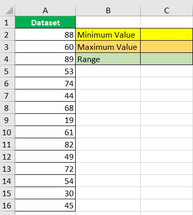
In column A, we’ll find an array of values.

We will be entering the formulae for the MIN and MAX functions in cells C2 and C3 respectively.

Finally, we will be entering the formula for finding the range in cell C4.

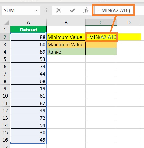
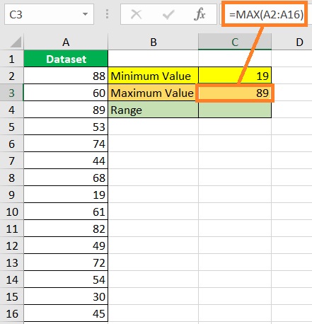
Find the dataset’s minimum value. Select a cell where you want to display the minimum value (which is cell C2 in our illustration). Then, enter the formula for the MIN function (in our illustration, the formula will be =MIN(A2:A16)).

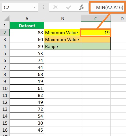
Press the ENTER key. The formula should return the dataset’s minimum value.

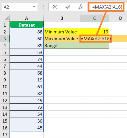
Find the dataset’s maximum value. Select a cell where you want to display the maximum value (which is cell C3 in our illustration). Then, enter the formula for the MAX function (in our illustration, the formula will be =MAX(A2:A16)).

Press the ENTER key. The formula should return the dataset’s maximum value.

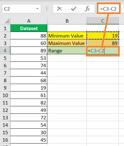
Finally, find the range by subtracting the minimum value from the maximum value. In our illustration, we will enter the formula =C3-C2 in cell C4 to find the range. Alternatively, you may skip the previous steps and calculate the range directly by entering the formula =MAX(A2:16)-MIN(A2:A16).

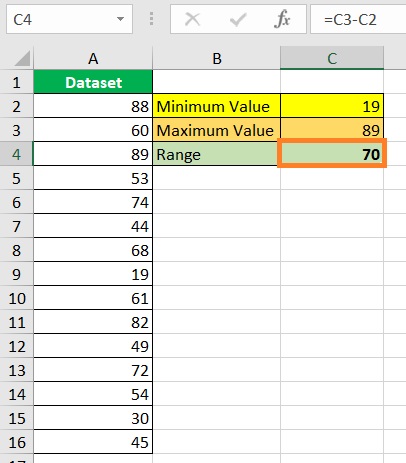
Press the ENTER key. You have successfully found the dataset’s range.

Use the SMALL and LARGE Functions to Calculate a Dataset’s Range in Excel

For the next method, we will be using the combination of the SMALL and LARGE functions.

Similar to the MIN and MAX functions, these two functions find the dataset’s smallest and largest values respectively.

However, they have a feature that the MIN and MAX functions don’t have.

The SMALL Function

The SMALL function finds the nth smallest value in a range of values.

Thus, you can use it to find the 1^st smallest value, or the 2^nd, 3^rd, 4^th, etc.

The formula to calculate it is as follows:

=SMALL(array,n)

Where,

array – refers to the range of cells from where you will be extracting the nth smallest value from

n – refers to the number’s position from the smallest value. For example, if you want the 1^st smallest value, n will be 1; If you want to find the 2^nd smallest value, n will be 2.

For example, you want to find 1^st smallest value in cells A2 to A11. The formula will be

=SMALL(A2:A11,1)

The LARGE Function

The LARGE function finds the nth largest value in a range of values.

Thus, you can use it to find the 1^st largest value, or the 2^nd, 3^rd, 4^th, etc. The formula to calculate it is as follows:

=LARGE(array,n)

Where,

array – refers to the range of cells from where you will be extracting the nth largest value from

n – refers to the number’s position from the largest value. For example, if you want the 1^st largest value, n will be 1; If you want to find the 2^nd largest value, n will be 2.

For example, you want to find 1^st largest value in cells A2 to A11. The formula will be

=LARGE(A2:A11,1)

Using the SMALL and LARGE Functions to Find a Dataset’s Range

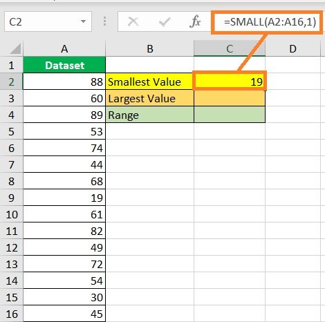
We will be using the same dataset with a little bit of change in the presentation:

In column A, we’ll find an array of values.

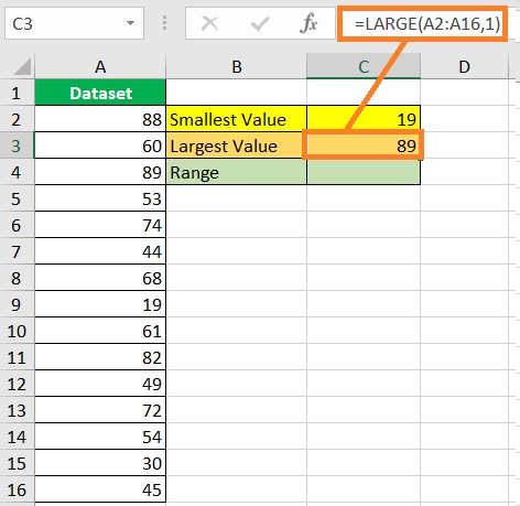
We will be entering the formulae for the SMALL and LARGE functions in cells C2 and C3 respectively.

Finally, we will be entering the formula for finding the range in cell C4.

Find the dataset’s smallest value. Select a cell where you want to display the smallest value (which is cell C2 in our illustration). Then, enter the formula for the SMALL function (in our illustration, the formula will be =SMALL(A2:A16,1)).

Press the ENTER key. The formula should return the dataset’s smallest value.

Find the dataset’s largest value. Select a cell where you want to display the largest value (which is cell C3 in our illustration). Then, enter the formula for the LARGE function (in our illustration, the formula will be =LARGE(A2:A16,1)).

Press the ENTER key. The formula should return the dataset’s largest value.

Finally, find the range by subtracting the smallest value from the largest value. In our illustration, we will enter the formula =C3-C2 in cell C4 to find the range. Alternatively, you may skip the previous steps and calculate the range directly by entering the formula =LARGE(A2:16,1)-SMALL(A2:A16,1).

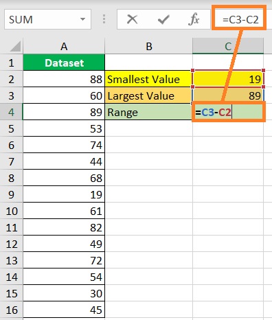
Press the ENTER key. You have successfully found the dataset’s range.

Calculate Conditional Range in Excel

In the newer versions of Excel (Excel 2019 and Excel 365), you can use the MINIFS and MAXIFS functions to find a dataset’s conditional range.

This is useful if you suspect that the dataset you’re working with has outliers.

For example, most of the values you’re working on range from 85 to 100.

However, there is one that has a value of 600, which is probably an outlier.

To ignore this outlier, you may use the MAXIFS function.

Suppose that the values are located in cells A2 to A16.

The formula to calculate the conditional range will be:

=MAXIFS(A2:16,A2:16,“<=100”)-MIN(A2:16)

This formula will ignore any value that exceeds 100 in its calculation.

Conclusion

And there we have. While there is no dedicated function for calculating range in Excel, there are still ways we can calculate it.

We can use the MIN and MAX functions, as well as the SMALL and LARGE functions.

I hope that you’ll be able to use your learnings here in your future endeavors!