Count Distinct Values with Excel’s PivotTableLearn how count distinct values in Excel with the PivotTable feature
Excel’s PivotTable feature is very useful for summarizing data.
It can make even a 10,000-entry dataset easy to read by just rearranging the rows and columns.
For example, let’s say that you’re working on a dataset that contains a record of all the transactions made by a store for the first quarter of the year.
With PivotTable, you can summarize the number of transactions, the total sales, or even the number of distinct customers or items.
It makes making certain reports much easier. Pretty nifty, huh?
Now, I’ve mentioned that you can the number of distinct customers or items with Excel’s PivotTable.
By that, I mean that you can count the number of distinct values from a dataset with the help of PivotTable.
Just to be clear, I mean distinct values and not unique values. Let me explain how these two are different:
Unique values – these are the values that only appear once in the list. In other words, there’s only one instance of a unique value in the column or row
Distinct values – these are the different values that appear in the list. A distinct value can have more than one instance in a column or row
To better visualize the difference, here’s an illustration:

That should make things clearer.
In this article, I’ll be showing you how to use Excel’s PivotTable to count the distinct values in a dataset. With this knowledge, you’ll be able to answer questions such as “How many distinct sales personnel made a sale?”, “How many distinct customers made a purchase in each store?”, “How many distinct items were sold?”, and etc.
Let’s get started.
Use Data Model With PivotTable To Count Distinct Values

From version 2013 and up, Excel gives the user access to data models. These can be used with PivotTable, which will provide more options if done so.
One of these options is “Distinct Count”.
What this does is count the distinct values in the source table or range.
Suppose you’re working with the following dataset (it has 40 rows, not including the column headers):
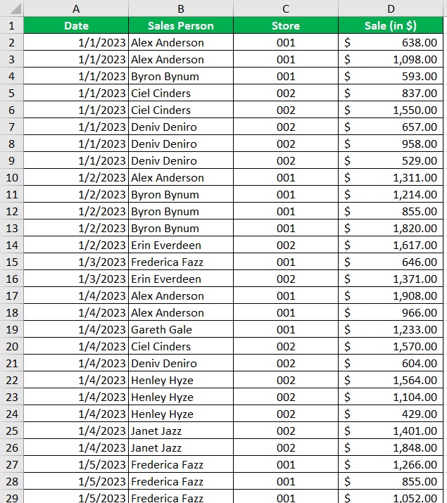
In it, you can find the daily sales of two stores for the first week of January, along with the salesperson who did the sales. You want to find out the following:
- The distinct number of salespeople per store; and
- The total number of distinct salespeople
How to Count Distinct Values
To do so, you’ll be using a data model with PivotTable.
- Select the table or range of cells that you’re working on (include the column headers). In our illustration, the range will be cells A1:D41.
- Open the Insert tab. On the left side of the ribbon, you should see the PivotTable button. Click on it. This will open the “Insert PivotTable from table or range” dialog box.

- In the dialog box, you should find the text box after “Table/Range” already filled in. This is because you previously selected it. If it’s not, select the table or range of cells that you want to source data from.

- Proceed to choose where you want the PivotTable to appear: (1) in a new sheet, or (2) or in the same sheet as the source data. If you choose the second option, you’ll have to select a cell where the first cell of the PivotTable appears.
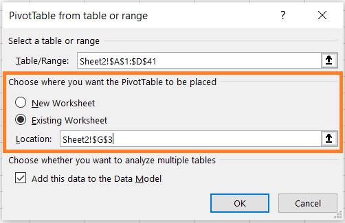
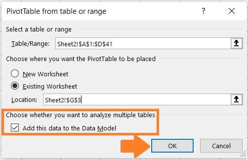
- Next, make sure to tick the box before “Add this data to the Data Model”. This is what allows you to count distinct values with a PivotTable. Click the OK button after doing so.
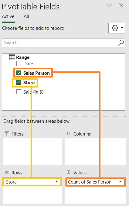
- Set up your PivotTable fields (via the sidebar that appears after clicking the OK button). In our illustration, we’ll be putting the Sales Person column in the Values field, while the Store column will go in the Rows fields. Since we’re only finding out the distinct number of salespeople, we don’t have to add anything else to the fields.
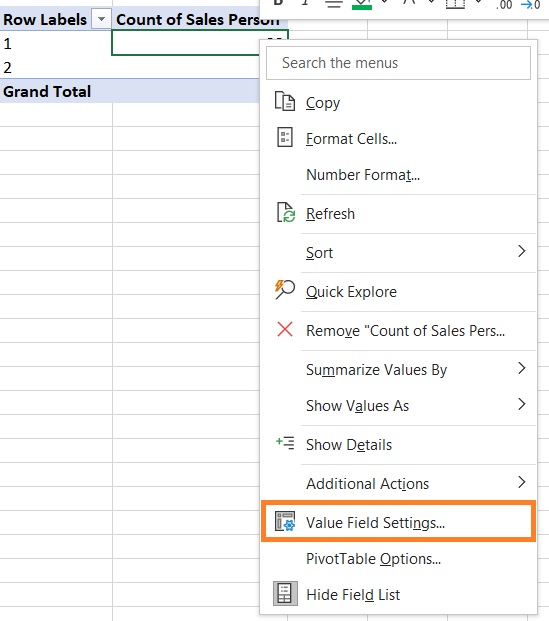
- Now go to your newly set up PivotTable. Right-click on any cell of the values field. This will show you a list of options. Select “Value Field Settings” from among them.
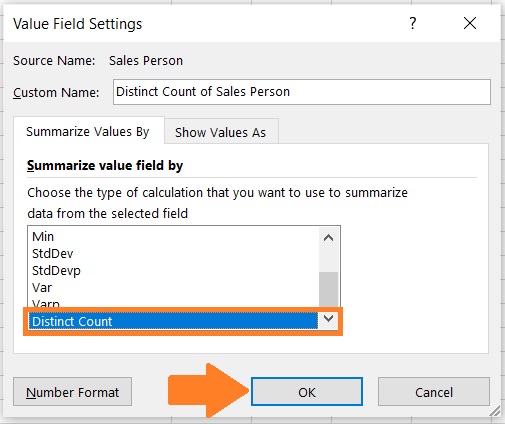
- In the resulting window, navigate until you find the “Distinct Count” option (usually at the very bottom of the list). Select it. Then, click the OK button.
- Your PivotTable should now show the number of distinct values. (I’ve formatted the table to make it more visually pleasing)

From the PivotTable, we can tell that:
- Store 001 has 5 distinct salespeople. Store 002 also has 5 distinct salespeople.
- In total, there are 10 distinct salespeople
Create A Helper Column (And Use The COUNTIF Function)
If you don’t have access to data models, you also won’t have access to “Distinct Count”.
But don’t worry for there’s another method you can follow. And you’ll be doing it with the help of the COUNTIF function.
The COUNTIF function counts from the range but with a certain condition.
Now, let’s say that you’re working with the same dataset. Only this time, you don’t have access to data models.
You still want get the following data:
- The distinct number of salespeople per store; and
- The total number of distinct salespeople
To do so, you’ll be enlisting the help of the COUNTIF Function
How to Count Distinct Values
- Create a new column. This will be your helper column. In our illustration, we name this column “Distinct Count”.
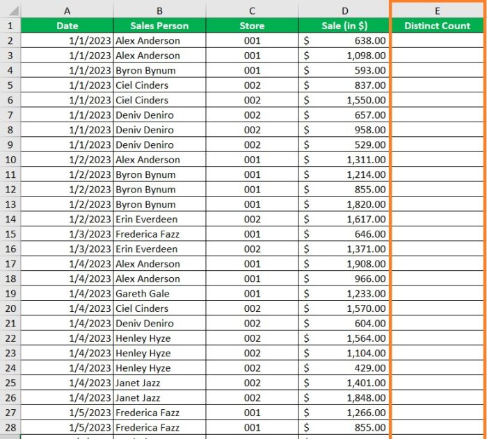
- In the first empty cell of the new column, enter the formula =IF(COUNTIF($B$2:B2,B2)>1,0,1). Press the Enter key after doing so.

- Copy the formula to the rest of the column (until the next empty row). The helper column should now be ready.
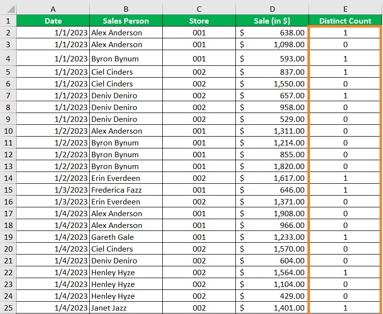
- Create a PivotTable using the dataset as your source. Then, set your PivotTable fields. In our illustration, we put the Store column in the Rows field and the Distinct Count column (our helper column) in the Values field.
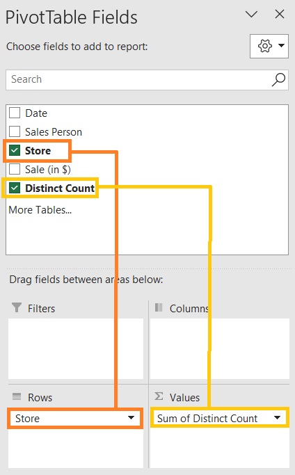
- Your PivotTable should now show the number of distinct values. (I’ve formatted the table to make it more visually pleasing)

From the PivotTable, we can tell that:
- Store 001 has 5 distinct salespeople. Store 002 also has 5 distinct salespeople.
- In total, there are 10 distinct salespeople
How the Formula Works
Now let’s talk about how the formula =IF(COUNTIF($B$2:B2,B2)>1,0,1) works.
The COUNTIF function is nested in an IF function. It counts the number of instances of the criteria in the selected range.
The range increases the further you go down the column because of how it’s structured. $B$2 is an absolute reference, while the second part is a relative reference which will be the same cell as the criteria cell.
Now, if the COUNTIF function counts more than 1 instance, the IF function will return a 0 value. If it counts less than 1 instance, the IF function will return a 1 value.
This way, only the first instance of the referred value returns a 1 value in the helper column. You can then use this column in your PivotTable to count the distinct number of values.
Use Power Pivot to Count Distinct Values in Excel
Another option for you to count distinct values is to use Power Pivot.
For the 2013 and up versions, Power Pivot is an inbuilt add-in that is deactivated by default.
For the older versions of Excel, you can download the add-in here.
To activate the add-in, open the File menu. Then, select options.


Then, in the Excel Options menu, select Add-ins. Next to “Manage”, select COM Add-ins, then click the Go button.
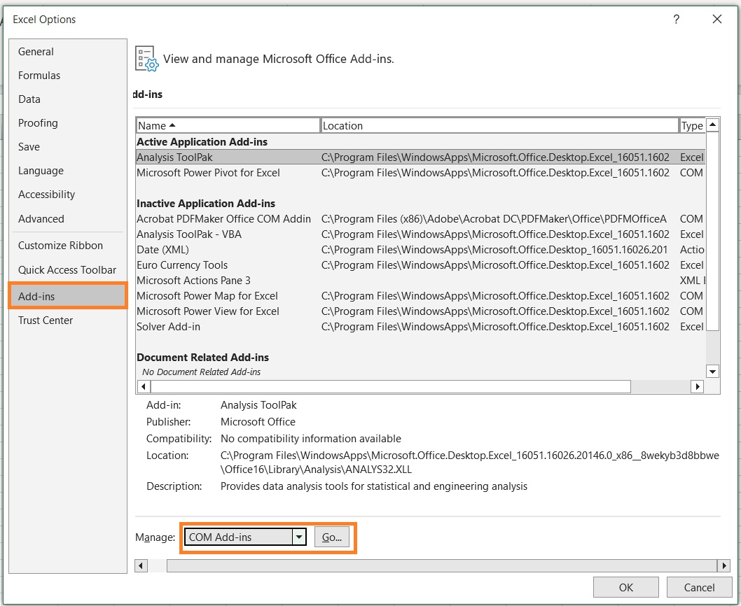
Then in the COM Add-ins window, tick the box before “Microsoft Power Pivot for Excel”, and then click the OK button.

This will load the Pivot Table tab to your Excel application.

How to Count Distinct Values
- Open the Power Pivot tab. On the left side of the ribbon, you should see the Manage button. Click on it. This will open the Power Pivot window.

- In this window, click on the From Other Sources button. This will open the Import Data Wizard.

- Navigate the wizard until you find the “Excel File” option. Select it, then click the Next button.
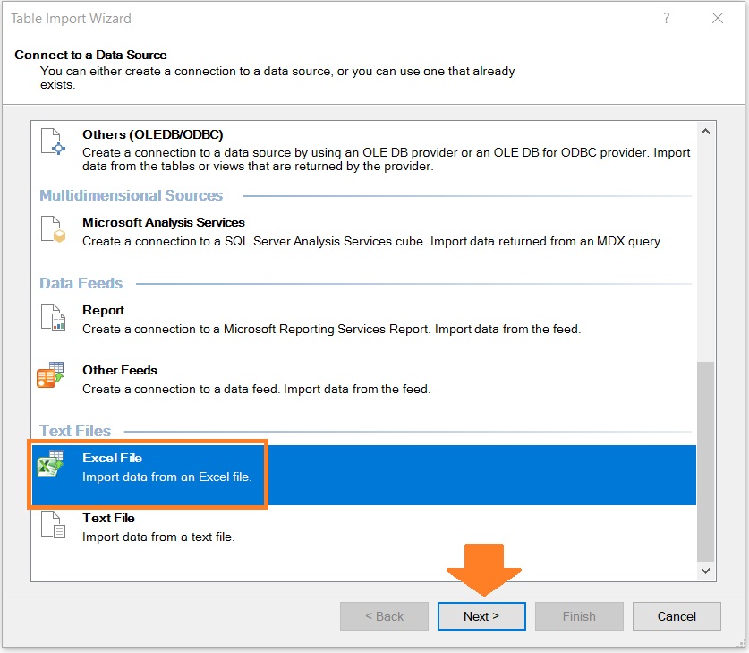
- Select the Excel file that contains the data that you’re working on. Then, tick the box below it if your data has column headers. Click the Next button after doing so.

- In the next window, just click the Finish button. This will import your data to Power Pivot.
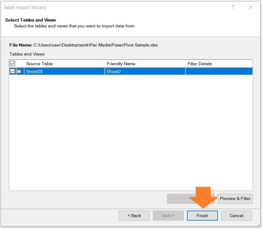
- Back in the Home tab of the Power Pivot window, click on the PivotTable button.

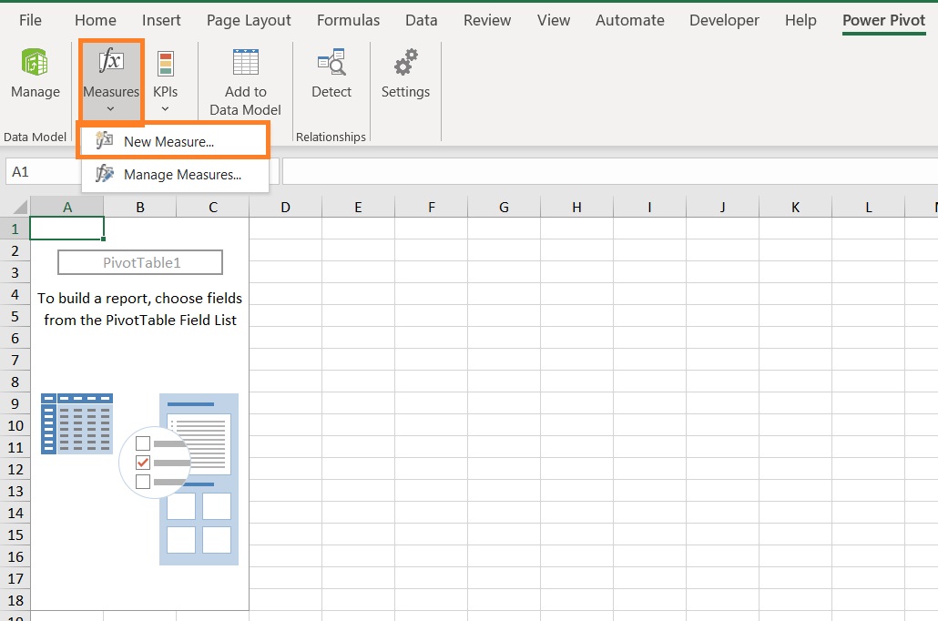
- The PivotTable will be created in Excel with the Power Pivot tab opened. Click on the Measures button then select New Measure.
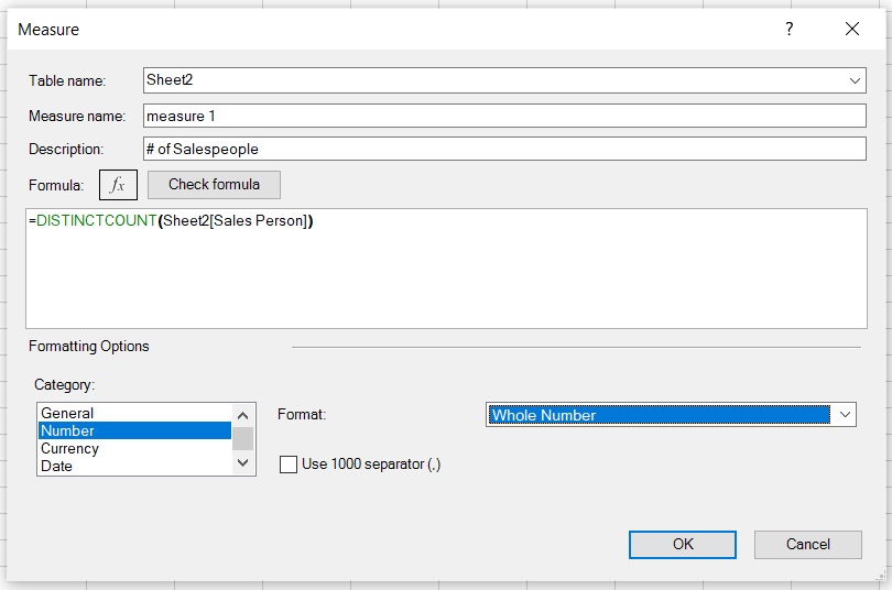
- This will open a window where you can add a new measure. Enter a description for the new measure, then enter the formula for it. Start with =DISTINCTCOUNT( then select the column that contains the values that you want to count distinct values from. Close it with a ), then click the OK button. You may set the Formatting Options to your liking.
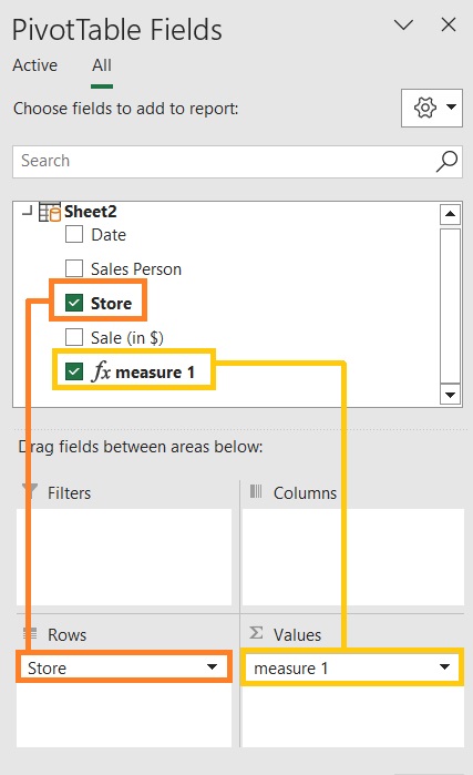
- The new measure should now be an option in the PivotTable. Set your PivotTable Fields, putting the new measure in the Values field.
- Your PivotTable should now show the number of distinct values. (I’ve formatted the table to make it more visually pleasing)

From the PivotTable, we can tell that:
- Store 001 has 5 distinct salespeople. Store 002 also has 5 distinct salespeople.
- In total, there are 10 distinct salespeople
Conclusion
And those are the different methods you can follow to count distinct values with PivotTable in Excel.
Which of the above methods do you prefer? Let me know in the comments.
