Apply Conditional Formatting to a Pivot Table in ExcelLearn how to properly apply conditional formatting to a Pivot Table in Excel

A Pivot Table is a very useful tool that aids in the analysis and summarizing of data. It can also provide another perspective on your data.

With it, you can create reports regarding the data you’re working on.

For example, let’s say that you’re working with a list of players for a game that has 4 servers.

With a pivot table, you can summarize how many players each server has.

And if the game has classes, you can also summarize how many players are of a particular class for each server.

Now let’s say that you already have your Pivot Table.

To make it more appealing, you highlight particular data.

For example, you highlight cells that have a value of 25 or above.

To do so, you’ll apply conditional formatting to your Pivot Table.

Alright. You have applied conditional formatting to your Pivot Table.

Cells that have a value of 25 or above are now highlighted.

That should be the end of it, right? Well, it probably isn’t.

You probably applied conditional formatting to your Pivot Table just like you would any cell on your worksheet.

But the thing is, applying conditional formatting to a Pivot Table is not as simple as that.

When you apply conditional formatting as is, it usually only gets applied to the selected cells.

Because of this, whenever a new column or row is added to your Pivot Table, conditional formatting won’t be automatically applied to it (the new column/row).

You’d have to reapply the conditional formatting to the new column/row.

But don’t worry. In this article, I’ll show you how to properly apply conditional formatting to a Pivot Table.

You no longer have to re-apply conditional formatting whenever a new row or column is added to Pivot Table if you follow these steps.

Use the Pivot Table Formatting Icon to Apply Conditional Formatting

For the first method, you’ll be using the Pivot Table Formatting Icon. If you’re wondering that is, let’s take another look at the Pivot Table example above:

You should now notice that there is a button inside the Pivot table (as shown above). This is the Pivot Table Formatting Icon. It appears whenever you apply conditional formatting to a Pivot Table. It will disappear whenever you perform another action (e.g. edit a cell, enter values, etc.).

Pivot Table Formatting Icon

When you click on The Pivot Table Formatting Icon, you will be presented with three options:

• Selected cells – the default option. This will apply conditional formatting only to the selected cells. If a new row or column is added to the Pivot Table, conditional formatting won’t be automatically applied.

• All cells showing “Count of Player ID” values – with this option, conditional formatting will be applied to all cells that show the Count of Player ID values, including the Grand Total column and rows. This option will automatically apply the conditional formatting to new rows or columns. It’s optimal if you want to include the Grand Total in the conditional formatting/highlighting rules.

• All cells showing “Count of Player ID” values for “Server” and “Class” – with this option, conditional formatting will be applied to all cells that show the Count of Player ID values in the column/row combination of Class/Server. This means that Grand Total won’t be considered in applying the conditional formatting. This option will automatically apply the conditional formatting to new rows or columns. It’s optimal if you don’t want to include the Grand Total in the conditional formatting/highlighting rules.

 

If you’re wondering how new rows/columns are added to a Pivot Table, it has to do with adding data to the backend (or reference table of the Pivot Table).

For example, if I add a new Server value in the backend (e.g. Erjis), a new row will be added.

If I add a new class (e.g. Cleric), a new column will be added. Note that for any changes to apply to the Pivot Table, you’d have to refresh it first.

How to Apply Conditional Formatting to A Pivot Table

Suppose you have already applied conditional formatting to your Pivot table as you would any cell, the Pivot Table Formatting Icon should appear:

• Click on the Pivot Table Formatting Icon. You will be presented with three options. Suppose you don’t want to apply conditional formatting to the Grand Total. The third option should be the best for you. Click on it.

• You have now successfully applied conditional formatting to the table. This conditional formatting will be automatically applied to new columns and rows.

Use the Conditional Formatting Button to Apply Conditional Formatting

Another option you can use to apply conditional formatting is to use the Conditional Formatting Button.

This button can be accessed via the home button. In the middle-right section of the ribbon, you will see the Conditional Formatting button.

Clicking on this button will present you with several conditional formatting options.

Now suppose you already applied conditional formatting to your Pivot Table:

However, you did so as you would any other cell in the worksheet. As such, you’d have to edit the conditional formatting settings.

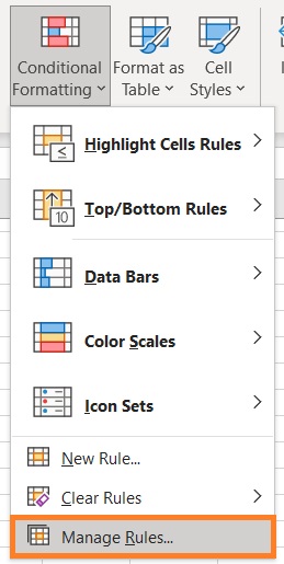
• Click on the Conditional Formatting button. It can be accessed via the home button. In the middle-right section of the ribbon, you will see the Conditional Formatting button.

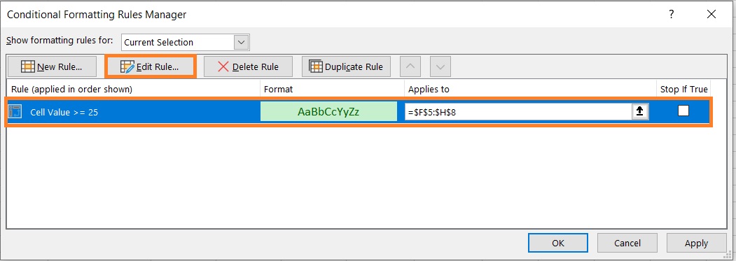
• Select Manage Rules from among the options. This will open the Conditional Formatting Rules Manager.

• Select the rule that applies to the Pivot Table. Then click the Edit Rule button.

• A new window should open. In this new window, you’ll see formatting options that are the same as what you’ll find by clicking the Pivot Table Formatting Icon. Select the third option for now and click the OK button.

• Close the Conditional Formatting Rules Manager. You have successfully applied conditional formatting to the Pivot Table. Let’s try it by adding a row to the pivot table:

Conclusion

If you want to automatically apply conditional formatting to any additions to your Pivot Table, doing it the usual way won’t do.

You have to make sure that it applies to the values in the Pivot itself and not just the selected cells.

If done properly, the conditional formatting should automatically be added to new rows/columns of the Pivot Table.