Apply the Accounting Number Format in ExcelWhat is the Accounting number format and how do you apply it in Excel?

Excel is an application that can be used for various purposes. That said, it’s most commonly used in the areas of business and accounting.

I mean, Excel has tons of functions that are ideal for business reporting.

You can even format your number strings into the currency format. It even has a specific number format for accounting which is the accounting number format.

Because of this, some small businesses may even use Excel to account for their books (e.g. general ledger, general journal, subsidiary ledger, etc.).

Accounting is a work of precision. Everything should balance out at the end.

And to get there, there should be as few mistakes as possible. Even a stray cent here or there can be an issue.

That’s why when you’re using Excel for accounting, you want to work with data that is easy to read and easy to look at.

Excel’s accounting number format is perfect just for that.

In this article, we’ll be discussing how one can apply the accounting number format in Excel.

We’ll also briefly explain what the accounting number format is.

How it is different from the currency format and the other number formats?

By the end of the article, you should be able to constantly and reliably apply the accounting number format to any numbers in the Excel sheet that you’re working on.

What is the Accounting Number Format?

In Excel, you can apply text or number formats for your data. For example, you can format numbers to look like currency, to show as fractions, etc.

You can also format numbers to appear as dates. There are two number formats that are particularly useful for business reporting and accounting.

These number formats are the currency and accounting formats.

These two number formats have their similarities.

By default, they add comma separators, a currency symbol, and two decimals points.

However, these two formats have a few differences that, while subtle, are enough to tell them apart.

Currency VS Accounting Format

Here’s a visual representation of how numbers look when the currency and accounting formats are applied to them.

Have you noticed the differences yet? Let me break it down for you:

• The currency symbol’s placement is different between the currency and accounting number formats. For the currency format, the currency symbol is located immediately beside the number. On the other hand, for the accounting format, the currency symbol is located on the very left side of the cell.
• Zero (0) is presented differently between the two number formats. With the currency format, zero is represented by the number itself (0) with a currency symbol beside it. With the accounting format, however, zero is represented by a dash or hyphen (-).
• Negative numbers are presented differently between the two number formats. With the currency format, negative numbers will have a hyphen or dash (-) before the currency symbol. This is also known as the minus symbol in mathematics. On the other hand, with the accounting format, negative numbers will be enclosed in parentheses.
• You have the option of including or not including the currency symbol with the accounting format. You don’t have this option with the currency format.

Why Use the Accounting Format?

In accounting, even the tiniest detail is important. Hence, you want to make the data you’re working with to be easier to look at.

What sets the accounting number format apart from other number formats is that it displays numbers in a consistent and easy-to-read manner.

The currency symbols and decimals will always be aligned no matter how small or large the number is.

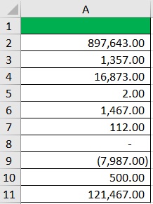
And yes, this applies whether the number is positive or negative. Just take a look at this:

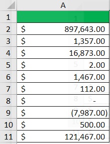
The presentation of data is aesthetically pleasing.

And with the consistent placements of the currency symbols and decimal points, it’s easier to accurately read the numbers.

Accuracy of data is important in accounting after all.

This is why the accounting number format is the preferred format when using Excel for accounting or business reporting purposes.

Apply the Accounting Format in Excel

The following are easy methods to apply the accounting format to your data in Excel.

Use the Accounting Button to Apply the Accounting Number Format

For the first method, we will be using the Accounting button.

This button can be found on the home tab, somewhere in the middle (it’s represented by a dollar sign):

If you want to exclude the currency symbol, you may want to use the button represented by a comma. It will format that cell into accounting format without the currency symbol:

How to Apply Accounting Format

Suppose that you have to work with the following dataset:

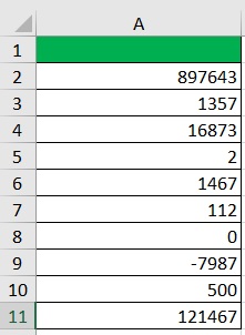
What you want to do here is apply the accounting format to these numbers so that they’ll be easier to work with.

• Select the cells that contain the data that you want to format.
• Open the Home tab. Somewhere in the middle, you should find a button represented by a dollar sign. This is the accounting button. If you want the dollar sign to be the currency symbol, click this button. If you want to select a different currency symbol, click the dropdown arrow next to the button, then select your preferred currency symbol.

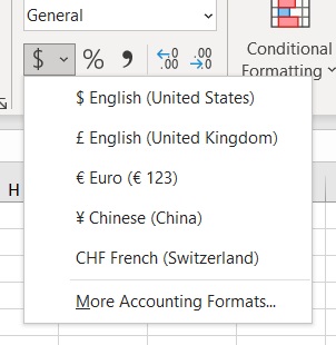
• The accounting number format should now be applied to your selection.

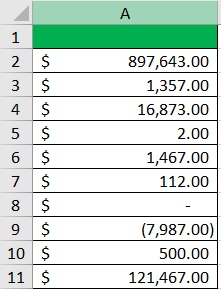
• [No currency symbols] If you want to apply the accounting format but exclude the currency symbol, you may press the button represented by a comma.

Use the Number Format Dropdown Menu to Apply the Accounting Number Format

For the next method, we will be using the format dropdown menu which can be accessed in the home tab. It can be found somewhere in the middle of the ribbon. By default, it will show ‘General’ and will have a down arrow on the right:

To access the dropdown menu, you’ll have to click on the down arrow.

How to Apply Accounting Format

Suppose that you have to work with the following dataset:

What you want to do here is apply the accounting format to these numbers so that they’ll be easier to work with.

• Select the cells that contain the data that you want to format.
• Open the Home tab. Somewhere in the middle, you should find a box that states the selected cell’s format (or the first cell in the case of a group of cells). By default, this will show ‘General’. There should be a down arrow on the right side of this box. Click on it to access the number format dropdown menu.

• From the options, select Accounting (click on it).

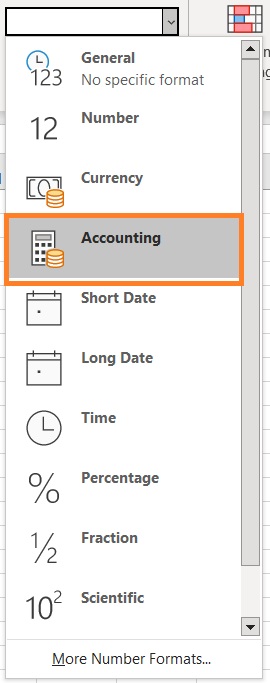
• This should apply the accounting format to your selection.

• If you want to select a different currency symbol, click the dropdown arrow next to the button represented by a dollar sign. Then, select your preferred currency symbol.

Use the Format Cells Dialog Box to Apply the Accounting Number Format

For the last method, we will be using the Format Cells dialog box.

This is a versatile and useful dialog box that lets us perform all formatting for our selected cell or cells all in one place.

To access the Format Cells dialog box, we will have to right-click on our selection and select the Format Cells option.

Alternatively, we can use the keyboard shortcut Ctrl + 1.

How to Apply Accounting Format

Suppose that you have to work with the following dataset:

What you want to do here is apply the accounting format to these numbers so that they’ll be easier to work with.

• Select the cells that contain the data that you want to format.
• Right-click anywhere on your selection. This should present you with a list of options. Select Format Cells from among them. This will open the Format Cells dialog box. (Alternatively, you may press the keyboard shortcut Ctrl + 1)

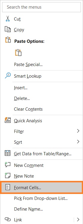
• In the Format Cells dialog box, open the Number tab. Then under ‘Category’, select ‘Accounting’.

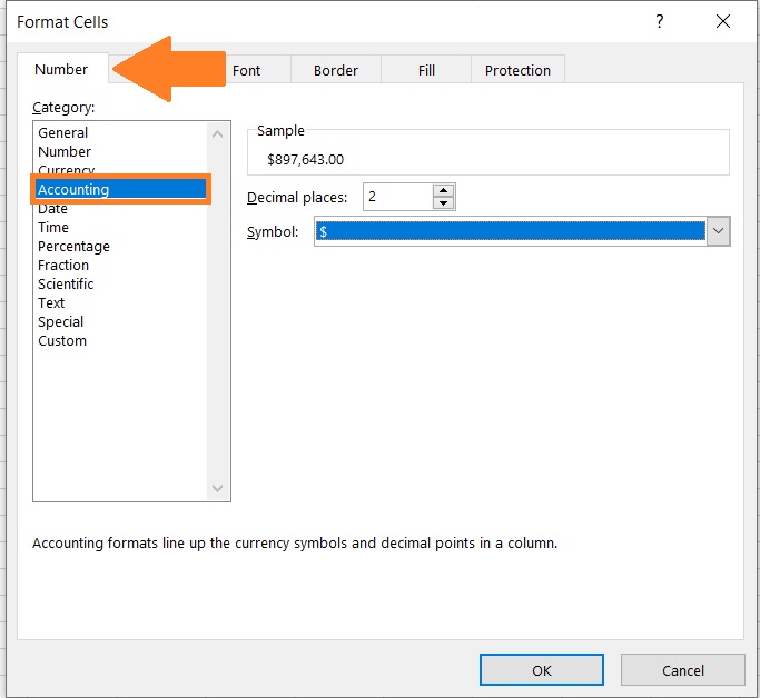
• On the right side of the dialog box, you should be able to see a sample of how the number would look after applying the accounting format. You can also increase or decrease places as well as select your currency symbol (or remove it). After customizing the settings to your preference, click on the OK button.

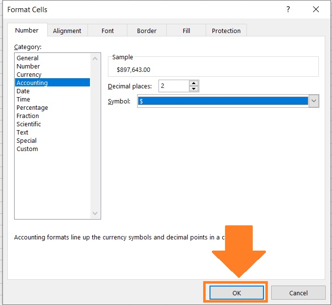
• The accounting format should now be applied to your selection.

Things to Keep in Mind When Applying the Accounting Number Format in Excel

• You can apply the accounting format to a blank cell. When you do so, any number added to the cell in the future will automatically have the accounting number format.
• The accounting number format only works for numerical values (as does any other number format).
• Applying the number format will not change the original value contained in the concerning cell/s. It only changes how the numbers look.
• You cannot remove the thousands separator (,) from a number if it’s in the accounting number format.
• The accounting format has decimal places of 2 by default.

And those are the different ways to apply the accounting number format in Excel.

I hope that you’ll be able to use your learnings from this article in your future endeavors.