Economic Order QuantityDefinition, Formula, and Examples for Inventory Management

Inventory management is a tricky endeavor.

You need to keep a lot of things in mind such as:

• How many units should be ordered
• The cost of holding stocks of products or materials
• The minimum level of inventory before the business could order new stocks
• The maximum capacity of your storage or warehouse facility
• Whether it is worth getting another warehouse or storage facility to house excess stocks; and many more.

Thankfully, there are many tools available that can help in inventory management.

With these tools, inventory managers can compute for the optimal reorder point, the ideal level of inventory, the minimum order and holding costs, etc.

Economic Order Quantity, or EOQ for short, is one of these tools.

After reading this article, you’ll be equipped with knowledge about EOQ: what is it, how it is computed, and how it can be applied to your business.

What is EOQ?

The cost of ordering inventory decreases as the ordering quantity increases.

This gives a business incentive to order in bulk rather than in small quantities.

However, this comes with a caveat. As the ordering quantity increases, the size of inventory also increases.

And as inventory grows, the cost of holding inventory grows too.

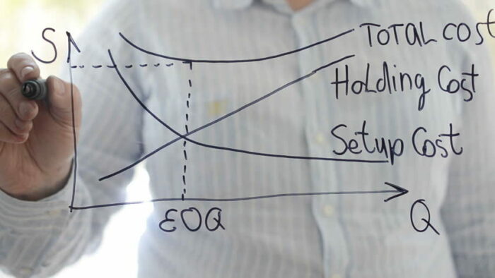
So the dilemma in inventory management is to find that sweet spot where ordering costs and holding costs coincide.

That’s where EOQ steps in.

Economic Order Quantity or EOQ refers to the optimal quantity a business should purchase per order.

This is to minimize inventory costs such as order costs, holdings costs, shortage costs, etc.

EOQ is one of the tools used in inventory management. To summarize, EOQ is an inventory management tool used to determine the optimal quantity and frequency of orders to minimize the cost per order.

EOQ was developed in 1913 by certain Ford W. Harris.

Its formula comes with assumptions as to the demand, order costs, and holding costs among other things.

The formula is presented as:

EOQ = √(2DS  ÷ H)

 

-or-

 

EOQ = (2 x D x S ÷ H)^1/2

Where:

D = Annual quantity demanded

S = Ordering cost

H = Holding cost

It should be noted that the resulting EOQ figure does not necessarily represent the cost of the purchased products themselves.

Additionally, it also does not represent the optimal reorder point (the minimum amount of inventory before the business restocks).

The EOQ figure only represents the optimal quantity of products to be ordered per purchase order to minimize inventory costs.

Components of the EOQ formula

To further understand the EOQ formula, let’s expound on its components:

Annual Quantity Demanded (D)

Annual Quantity Demanded (D) refers to the volume/quantity of demand that the business expects for the year.

The figure for the annual demand can be based on a business’s historical data.

For example, if the previous years saw a constant growth of 10% in demand, then it can be assumed that this year’s annual demand will be 110% of the previous year’s demand.

The EOQ formula assumes that the demand for a business’s products remains constant throughout the year.

This means that seasonal changes or unaccounted fluctuation in demand are not considered in the EOQ formula.

Ordering Cost (S)

Placing an order often comes with a cost such as the following:

• The cost to prepare a purchase order
• The cost of delivery
• Inspection fees
• The cost to prepare and issue payment to the supplier
• The cost of receiving the order

We refer to these costs as ordering costs.

It can be variable, fixed, or a mix of both.

The EOQ formula assumes that the ordering cost will remain constant throughout the year.

This means that it does not account for discounts and fluctuations.

Holding Cost (H)

As with placing an order, holding inventory comes with costs too.

Maintaining a storage facility or warehouse isn’t free after all.

Holding cost can be a direct cost that is incurred whenever a business has to hold inventory (e.g. storage fees, salaries and wages of warehouse employees, etc.).

It can also be an opportunity cost – when spending money for inventory, you forego the income you can potentially earn by investing the money elsewhere.

Holding cost is often expressed as a cost per unit.

If holding cost is treated as an opportunity cost, it is expressed as a cost per unit multiplied by the interest rate.

Put into formula form, it will look like:

H = i x C

Where:

               H = Holding cost

               i = interest rate or carrying cost

               C = cost per unit

As with the other components, the EOQ formula assumes that the holding cost remains constant throughout the year.

This means that fluctuations in holding costs won’t be accounted for.

Assumptions when calculating EOQ

As we were breaking down the components of the EOQ formula, several assumptions were mentioned.

To reiterate:

• The EOQ formula assumes that demand for your business’s products will remain constant throughout the year. Fluctuations in demand and seasonal changes won’t be accounted for.
• Ordering costs will remain constant throughout the year. Discounts and other changes (e.g. increase or decrease in transfer costs, inspection fees, etc.) won’t be accounted for.
• Holding costs will remain constant throughout the year. This means that any increases or decreases in holding costs won’t be accounted for. For example, if the salaries and wages of warehouse employees increase, it won’t be accounted for in the computation of EOQ

In addition to the above assumptions, the EOQ formula also assumes the following:

• The business does not have any safety stocks.
• The business will only reorder once inventory is fully depleted or time it so that when the new stocks arrive, there is no inventory on-hand.
• Customers won’t order more than the available inventory.
• The business’s storage facility or warehouse can accommodate the EOQ

Examples of calculating EOQ

Allison is one of the inventory managers of a company that operates a retail store.

The company is planning to stock a new product.

The company’s top management assigns Allison to manage the inventory of the new product.

The company is expecting that the annual demand for the new product will be 100,000 units.

As per the supplier, the expected ordering cost would be $20 per order.

The holding cost is expected to be $4 per unit.

Allison wants to know the optimal quantity of units to be ordered per purchase order so that the company can save on ordering and holding costs.

To get the figure, Allison computes the EOQ of the new product:

EOQ = √(2DS  ÷ H)

EOQ = √((2 x 100,000 x $20) ÷ $4)

EOQ = √($4,000,000  ÷ $4)

EOQ = √1,000.000

EOQ = 1,000

After calculation, Allison finds out that the optimal quantity per order is 1,000.

With this in mind, Allison places an order from the supplier for 1,000 units of the new product.

She also notes to the purchasing team to only order in quantities of 1,000 for the new product.

Allison then presented the following data to the top management to show a comparison of different order levels and why it is optimal to order 1,000 units of the new product per order:

Quantity Per Order	Frequency of Orders	Total Ordering Costs	Total Holding Costs	Total Cost of Ordering and Holding Inventory
900	111	$2,220.00	$1,800.00	$4,020.00
1,000	100	$2,000.00	$2,000.00	$4,000.00
1,500	67	$1,340.00	$3,000.00	$4,340.00

Allison convinces the top management and is commended for a job well done.

Let’s have another example.

Dave is operating an ice cream shop. Every year, he orders 4,000 gallons of milk to accommodate annual demand.

Each time he places an order for milk, he incurs $20 in ordering costs.

The cost of holding a gallon of milk amounts to $4.

Currently, Dave is ordering in quantities of 100 gallons per order.

He recently heard from Allison, a friend of his, about EOQ and wondered if he’s ordering the right amount per order.

Allison helps Dave by computing the EOQ for gallons of milk:

EOQ = √(2DS ÷ H)

EOQ = √((2 x 4,000 x $20) ÷ $4)

EOQ = √($160,000 ÷ $4)

EOQ = √(40,000)

EOQ = 200

Allison relays to Dave that he should be ordering in quantities of 200 gallons of milk instead of 100 gallons.

Doing so would save Dave money.

However, that did not convince Dave. So, Allison computed for the total annual inventory cost of ordering in quantities of 200 gallons and 100 gallons.

To compute the total annual cost, Allison uses the following formula:

Total Annual Cost = (D ÷ Q x S) + (Q ÷ 2 x H)

Where

               D = Annual quantity demanded

               Q = Quantity per order

               S = Ordering cost per order

               H = Holding cost per unit

 Allison first computes the total annual cost for orders in quantities of 100 gallons:

Total Annual Cost = (D ÷ Q x S) + (Q ÷ 2 x H)

Total Annual Cost = (4,000 ÷ 100 x $20) + (100 ÷ 2 x $4)

Total Annual Cost = $800 + $200

Total Annual Cost = $1,000

Allison then computes the total annual cost for orders in quantities of 200 gallons:

Total Annual Cost = (D ÷ Q x S) + (Q ÷ 2 x H)

Total Annual Cost = (4,000 ÷ 200 x $20) + (200 ÷ 2 x $4)

Total Annual Cost = $400 + $400

Total Annual Cost = $800

As per Allison’s computations, the total annual cost for orders in quantities of 200 gallons is $800 which is $200 less compared to that of 100 gallons which is $1,000.

Allison finally convices Dave. He will start ordering milk in quantities of 200 gallons per order from now on.

How EOQ can help you and your business

The main reason why you should be using EOQ for your business (assuming that it maintains inventory) is for improved profitability.

By finding the optimal order quantity, you can save up on ordering and holding costs which ultimately translates to higher income.

The following are some of the other benefits you get from using EOQ

• Less probability of overordering or underordering – by knowing the optimal order quantity, you are less probable to underorder or overorder. By not overordering, you save up on holding costs and you’d also have more available cash to put on other investments. By not underordering, you won’t be losing on potential sales due to insufficient stocks.
• Less waste and inventory obsolescence – a more optimized ordering scheme allows for optimized inventory management. This potentially removes the chance of inventory obsolescence, which is especially useful for businesses that stock perishable products
• Decrease storage costs – when your ordering matches with customer demand, you probably won’t have any problem in zeroing out your inventory.
• Improved order fulfillment -if you know your EOQ, you can plan your inventory to meet your customer’s demands. You can make sure that you have a product on hand if a customer demands it. This could translate to more customer satisfaction further resulting in more sales.

Limitations of EOQ

The very first limitation of EOQ is its assumptions: demand, order cost, holding costs will all remain constant throughout the year.

This makes it nearly impossible to account for events that can cause changes in these variables.

Case in point: the recent global pandemic.

COVID-19 brought about a disruption in the normal operations of businesses.

The EOQ formula cannot account for such uncertainties.

To remedy this, EOQ must be reviewed whenever there is anything that can significantly affect its components.

Another limitation of EOQ is that it does not account for seasonal changes and their effects on perishables.

For example, the EOQ of a certain perishable is 1,000.

The perishable has a shelf life of 30 days.

If there happens to be a month or two where demand is less than 1,000, then the business will have expired inventory.

The EOQ formula cannot account for this.

The EOQ formula does not account for discounts granted for ordering a certain quantity of products.

However, there is a workaround for this. First, compute the EOQ for the undiscounted ordering cost.

Then compute the EOQ for the discounted ordering cost and see if it is feasible. You then compare the two EOQ and assess which one is better.

The EOQ formula assumes that the business only replenishes inventory when it is zeroed out (or when it is about to be completely depleted by the time the new stocks arrive).

It also assumes that inventory can be replenished in just one shipment.

However, this is not always feasible for some businesses.

They might require a minimum amount of inventory as safety stocks.

To remedy this, EOQ must be used in conjunction with another inventory management tool which is the reorder point (ROP).

To make the most out of EOQ, it is recommended that it’d be used in conjunction with other inventory management tools to make up for its limitations.