How to Use the Google Sheets Indirect FunctionComplete Guide


Unlike the Address Function in Google Sheets which tends for the address of the cell to be returned in text format, the INDIRECT function works the opposite way – the cell address is taken as a text and is returned as a cell reference.
The Indirect Function uses a text string for the cell address in finding the cells.
The use of a text string actually provides many advantages which are highlighted in the next sections of this article.
Indirect Function Syntax
Here’s the syntax to use when using the indirect function:
INDIRECT(cell_reference_as_string, [is_A1_notation])
Where:
- Cell_reference_as_string – this is the address of a cell in a text format. This should be enclosed in quotation marks (“ “) because it is a text string. The quotation mark is not necessary when a cell is referenced in the text string.
- is_A1_notation – this is only optional. What this does is instruct the function with regard to the cell address notation. For example, B1 refers to column B row 1. So if the notation is B1, it refers to the cell in column B row 1. Another way to reference a cell would be R2C2 which refers to B2 because the second column is B and the second row is row 2. The default value for B2 is TRUE but in case you wish to get the R2C2 notation, you have to specify it as FALSE.
The Indirect Function: How to Use
It might be difficult to understand how to use the indirect function by simply defining it and providing a syntax.
Below is an illustration to help you understand it fully:

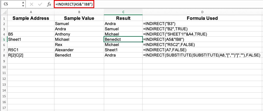
Let’s go through each of the formulas used to better demonstrate what the results would be using the different functions.
Formula # 1
The first formula used is very straightforward – I am instructing that the result be what is the date inside cell B3, which Andra.

Formula # 2
Here, I am doing the same thing I did in the first formula, where I want the result to be the same as that of cell B2 which is Samuel.
The difference is that I have included the annotation for A1 by indicating TRUE.
This is only optional. Had I entered FALSE, the annotation would have been R1C1 instead of A1.

Formula # 3
The third formula uses a text string that is concatenated.
It instructs exactly what cell is being referenced.
For example, in the formula, ‘=INDIRECT(“SHEET1!”&A4,TRUE) the string refers to the cell A4 that is in Sheet1.
A4 also references B5 which contains Michael.
The optional part of the formula – True – refers to A1 notation.

Formula # 4
Here, it basically does the same thing as the one in Formula # 3 except for one thing – it has added Sheet1!
B8 and has referenced A5 which also references sheet 1.
The result still returns B8 which is Benedict.
Formula # 5
Here, the formula does not use the A1 notation which is why you will be able to find FALSE at the end of the formula and the referenced cell which is R5C2 – the fifth row of the second column.
The result here returns Michael.
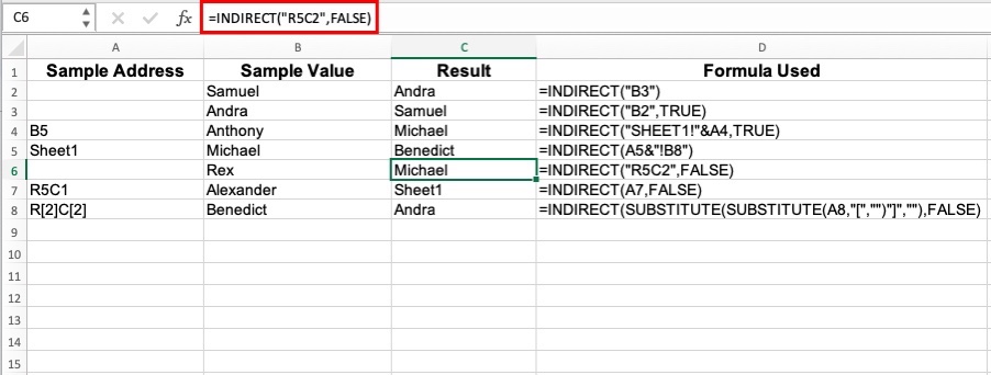
Formula # 6
In the sixth formula, notice two things here: the cell is directly referenced which is A7 but in this referenced cell, it is not in the A1 notation format so we add FALSE in the formula.
This then returns the result Michael which is what the fifth row and second column contain.

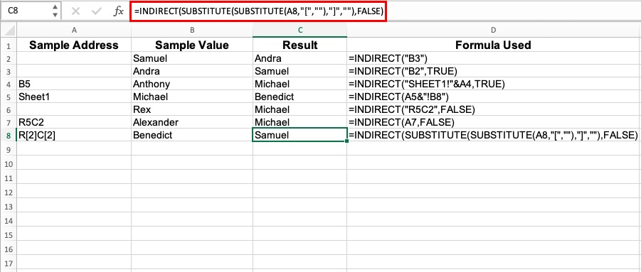
Formula # 7
You will notice that we used the substitute function here.
This is because the data in cell A8 is in a different format which our formula will not be able to recognize.
The use of substitute ensures that R[2]C[2] will become R2C2 which will now be recognized as the second row in the second column – Samuel.
Cell Range Maintained in a Formula
One of the many great benefits that the Indirect Function provides is that no matter how many rows or columns you add when a cell range is referenced, it does not change.
The table below shows the difference between using an Indirect Function with the Sum Formula and the Sum Function.
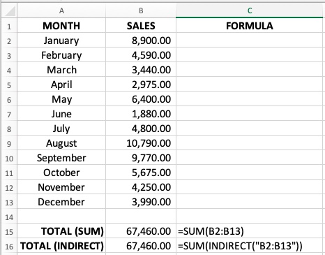
Here you will notice that the total is the same. Where the difference comes into play is when you add rows or columns to the cell range.
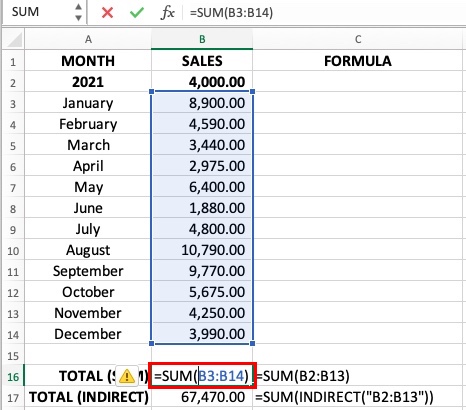
Notice that when we added a row above January, the Sum Formula adjusts automatically and it has now become B3:B14.
This did not affect the Indirect formula – it has stayed the same.
Use in Name Ranges
If you wish to refer to named cells instead of numerical values in a cell, you can do this by following the below steps:
- Select the cells you wish to name. For our example, we will refer to cells B2:B13.
- Go to Data and then click on Named Ranges.
- Give your selected cells a name. In this example, I have named it Months.
Now that I have named the cell range, I can now use the Indirect Formula. See the table below:

The formula used here is =SUM(INDIRECT(“Months”)).
When using the named range in the formula, it will automatically reference the value of the cells in B2 to B13.
Use to Reference to Other Sheets
The Indirect Function can also be used to reference cells that are located in a different worksheet.
To do this, let’s illustrate it below for a clearer example.
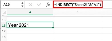
I have added Sheet 2 to my worksheet and entered in Cell A1 the text “Year 2021”.

Going back to Sheet 1, I can reference the data in Sheet 2 using the below formula:
=INDIRECT(“Sheet2!”&”A1”)
The advantage of using this formula is that you have multiple sheets and you need to pull different information from different sheets.
In case you have referenced the worksheet, you can simply edit the sheet number directly in the formula bar.
Use Indirect Formula with MATCH
The use of the Match function with the Indirect function results in your cells having dynamic ranges.
To combine both, let us use the below formula to executive the Indirect and Match functions:
=INDIRECT(“B” & MATCH(B15,A:A,FALSE) & “:B” & MATCH(B16,A:A,FALSE), TRUE)
The result will then be shown as the one below:

In using the above formula, the start and end months have been specified. Using the MATCH function, it finds the months that I have specified in the range and determines the rows where they are located.
Using the indirect function, the months in between the specified months are also included and this gives me sales from January to September.
This setup will allow me to change the months as needed.
This can also be set up to include the SUM formula to get the sum of all specified cell ranges.
Use Indirect Formula with TABS
When you want to get consolidated data from the different tabs in a spreadsheet, the Indirect Function will help you do this fast.
Take the below example. I have different tabs for each of the month’s sales with weekly sales summaries.
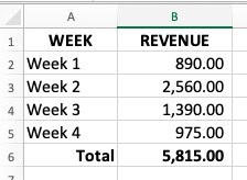
With our summary tab, the total for each month can be summed up.
The longer method would be to manually copy and paste the totals but there is an easier way.
You can instead use the Indirect Function:
=INDIRECT(A2&”!B6”)

This formula can only work if the total sales for the month are located in cell B6 for all of the tabs.
The formula instructs Google Sheets to look at B6 for all of the tabs and the great thing about this is that any change in the tabs referenced is reflected in the summary in real time.