Excel Wildcard CharactersWhat Are They & How To Use Them Properly


Wildcards in Excel are special characters that can help in finding text values that are similar but not quite identical.
There are three Excel wildcard characters.
These are the question mark, tilde, and asterisk.
The question mark is used to represent a single character, whereas the asterisk is used for several characters.
Alternatively, the tilde cancels the effect of wildcards when it is placed before them.
Basically, it will turn the wildcard into a literal character, such as turning a wildcard * into a literal *.
These characters are useful when searching or replacing content, as well as in some conditional formatting rules.
The Three Types of Excel Wildcard Characters
There are three types of wildcard characters, and we will explain these next.
The Asterisk (*)
The asterisk can be used to match strings of any length. As an example, you could put “ma*,” and it could match words such as “maple,” “match,” or “man.”
The Question Mark (?)
You can use the question mark to match any one character. As an example, you could put “?ake,” and it might match “cake,” “bake,” or “make.” Another example would be putting “b*t,” which might find “bat,” “bit,” or “bet.”
The Tilde (~)
The tilde cancels the effect of a wildcard and can be used to find a wildcard character that is being used as text. Suppose you wanted to look for text that contains an asterisk that is not being used as a wildcard. If you were searched for contestant~*, the results would show cells with the word contestant. However, if you searched for contestant*, the results would show any cells that begin with contestant*.
Wildcard Character Examples
We will now show a few examples of how to use these wildcard characters.
Example One – Using an Asterisk
In this first example, we will show how you can use an asterisk to match any number of characters you choose in a sentence.
In this example, we will use the data below.

In our data, we have the names of sales representatives. Several of our sales representatives have the first name, Cindy.
Now, if we want to see how many of our sales representatives are named Cindy, we can use the wildcard asterisk. First, open the COUNTIF function. Then, select your range.
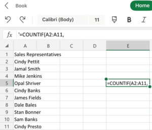
In order to have the number of people named Cindy counted, we put the criteria in the argument.

Now, all the names containing Cindy will be counted.
Example Two – Partial Lookup Using a Wildcard Character With VLOOKUP.
If we want to use VLOOKUP to look up values in data, we will need to have an exact look_up value, which will be matched to retrieve the data. It will not work correctly if you supply it with an approximate match. But you can do this by using wildcard characters.
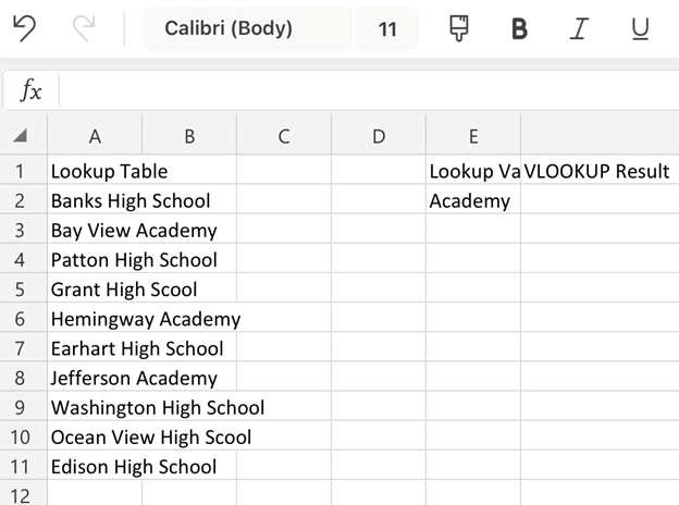
Suppose we are looking for a certain school in a list of schools, we are not sure of the name of the school, but we know it contains the word academy, not school. If we just used part of the name with VLOOKUP, it would not find the school. Here is the data we will use.
The lookup table is in column A, and the lookup values are in column E. So, we will need to use wildcards, and we will show you how to do this.
Start by placing this formula in cell F2 and drag it to the other cells.
=VLOOKUP(“*”&E2&”*”,$A$2:$A$11,1,TRUE)
Notice that we placed two asterisks in the formula. These asterisks show that anything between the wildcard characters is a match and should be returned as a result. In our case, it should show all the schools with Academy in their name.
Example Three – Find and Replace
Another common way wildcard characters are used is to find and replace data. We will use the data below.

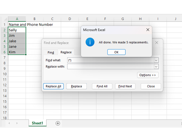
Suppose we have a list of peoples’ names and phone numbers that were entered in the same cell, but we only want the names. We can use wildcard characters to keep the names and not the phone numbers.
First, we will select the data in which we will be replacing text. Then, we go to “Find & Select” in the “Home” tab and choose “GoTo,” which will bring up a dialog box.

Now type “(*)“ in the “Find What” box, and allow the “Replace With” box to remain blank. Now we choose “Replace All,” and we will have the names with no phone numbers.
Example Four – Count Non-blank Cells that Contain Text
In this example, we will show how to use an Excel wildcard character with the COUNTA function so that it will only count cells with text in them.
This overcomes the problem the COUNTA function has of counting cells that look blank but have =”” in them.
Here is the formula to use to count only cells that have text values.
=COUNTA(A1:A11,”?*”)
If your cells have text and numbers, the following formula will work.
=COUNTA(A1:A11)-COUNTBLANK(A1:A11)
These formulas ensure that Excel will only count cells that have a minimum of one character in them.
Conclusion
We have explained three different wildcard characters, the “*,” the “?,” and the “~.”
We also gave a few examples using some of these characters.
Although there are many additional ways in which you can use these wildcard characters, such as for MATCH() or SUMIF(), and you will likely find that there are many more situations in which wildcard characters can be useful.