How To Use VLOOKUP with Multiple CriteriaEasy Step-by-Step Guide with Screenshots

Last Updated: February 9, 2023

Microsoft Excel is an incredibly powerful tool for managing, organizing, and analyzing data, and as such, it includes many tools for users to analyze and interpret stored data.

Among the many functions that Excel holds to make it easier for users to work with their data, VLOOKUP is one of the most powerful.

VLOOKUP allows users to find the data they are looking for within a table or range by row, opening up the potential to sort through hundreds or thousands of pieces of data within a column quickly or easily.

However, in its basic form, the VLOOKUP function has one significant limitation, and this is that it will only look for one value, which can be quite a drawback when you need to search for a result based on multiple criteria.

Though this is not a capability that VLOOKUP provides by default, it is possible to do, and here we will show you how.

First, however, we will take a look at how the VLOOKUP function works and what information you will need to use it.

What Is VLOOKUP and How Can It Be Used?

VLOOKUP, which stands for vertical lookup, is one of Excel’s built-in functions which allows users to search for a specific value vertically across a worksheet and return the applicable row.

This is an incredibly valuable function when one needs all of the data contained in a row but only as part of the information.

Though in many cases, the newer VLOOKUP function, which can work in any direction, has surpassed this tool in functionality, those with older versions or with specific needs may still choose to use VLOOKUP. The syntax for this function is:

=VLOOKUP (search value, range to search, column number, [approximate or exact match])

In order to fill out the values in this syntax and use the VLOOKUP function, you will need a few specific pieces of information. This includes the :

Search Value: This is the value you want Excel to search for or “lookup.”
Range to Search: This is the range where your search value is located. In order for VLOOKUP to work effectively, the search value should be located in the first column of the specified range. This means that if the search value you wish to locate is cell B22, then your search range should start with column B.
Column Number: This is the column number in your search range that contains the return value. This means, for example, that if your range is C5:E7, you would include C as the first column, D as the second, and E as the third.
Approximate or Exact Match: These two options determine whether the search will return only an exact match or an approximate match. Set this value to “True” for VLOOKUP to return approximate matches and “FALSE” for exact matches. If you do not include anything under this value, then Excel will set it to “TRUE” by default.

When these values are put together in the correct syntax, it will create the powerful search function VLOOKUP. Now let’s see how it can be used to search with multiple criteria.

How To Use VLOOKUP With Multiple Criteria

When using VLOOKUP, there are many situations when it can be useful to extract particular data from a range based on multiple criteria.

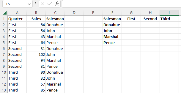
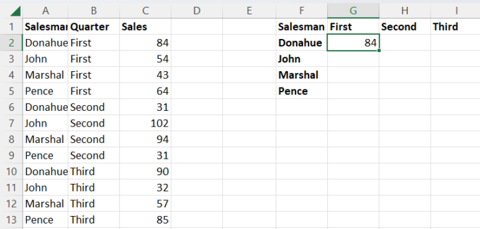
For example, consider a data set containing information on the sales each member of a group of salesmen have made in the first three quarters of the year.

With this information, applying the VLOOKUP function to acquire the sales each employee has made in each of the first three quarters would be difficult.

Now, in most cases, using a Pivot Table to store and work with the data may be a better idea for making it easier to analyze and work with data like this.

However, this is not always an option, such as when you are working with data owned by another author.

So, in these cases, VLOOKUP may be the best tool at your disposal, and there are two ways that you can use it to evaluate data using two criteria.

These include creating a helper column and using the CHOOSE function.

Evaluating Multiple Criteria in VLOOKUP With Helper Columns

Since VLOOKUP is unwilling to natively evaluate multiple criteria, we need a workaround, and one of the easiest is to create a helper column.

This column can be added next to your existing source data and will be used to join multiple fields, and in this case, criteria, together in order to help VLOOKUP find the correct values.

This is relatively fast and easy to do and can make it easier to analyze the source data if you want to check for accuracy.

It also makes it far faster and easier for those with less experience working with Excel functions when compared to using array functions.

This simply means it is more limited, but in most cases, it will get the job done.

With this method, we will create a new “helper” column, which will create a unique identifier that VLOOKUP will use to find your results.

In this way, we can use multiple criteria in VLOOKUP without needing any complex workaround.

In our data, we want to know how much each salesman has sold per quarter for the first three quarters of the year and place it in the appropriate cells.

To do this, we will first create a helper column and then use VLOOKUP to search based on these two criteria.

Create a helper column next to your data

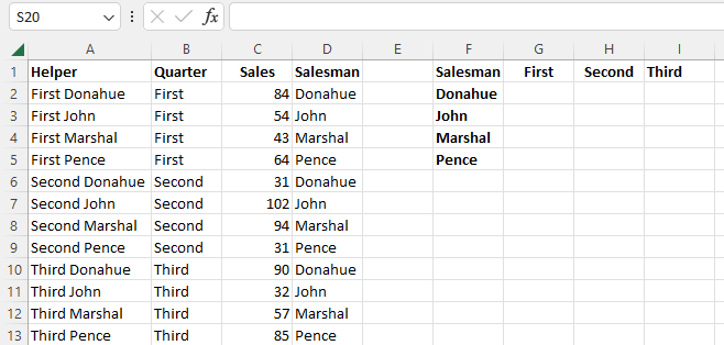
Now combine the relevant criteria from the two lookup columns into the helper column. In our case, we will use the formula: =B2&” “C2. Simply substitute your own cell values appropriately. This will concentrate the cell value into the helper column to create a unique identifier that VLOOKUP can use in its search.

Now enter the standard VLOOKUP formula with both criteria included in the search value with a space separating them. In our case, =VLOOKUP(“First Donahue”, A2:D13,3,FALSE).

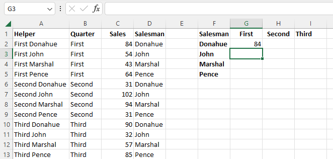
VLOOKUP will use the helper column to locate the data based on the two criteria and return the specified value.
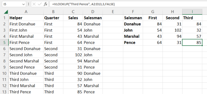
Now, this can be copied for all of the remaining cells.

As you can see, this is a relatively simple procedure to search by two criteria, and in theory, it is not limited to only a pair of criteria.

However, keep in mind that the search value is limited to only 255 characters.

Another drawback to this procedure is that it consumes valuable worksheet space and clutters its appearance in order to create the helper column.

For those that would like another workaround, there is another method that we will look at next.

Evaluating Multiple Criteria in VLOOKUP With the Choose Function

If worksheet space is at a premium or you simply would prefer to avoid the clutter of helper columns, there is an alternative, and this is through array formulas.

In these cases, the CHOOSE function can be used within the VLOOKUP formula to allow searches with multiple criteria as well.

The resulting array formula will provide us with the same result judging the values within the search range by multiple criteria without all the clutter.

In order to do this, we will need to use a more complex formula which is:

=VLOOKUP(CONCATENATE($F$2, $G$1),CHOOSE({1,2},$A$2:$A$13&” “&$B$2:$B$13,$C$2:$C$13),2,TRUE)

So, here is how this method can be used considering the same example as above.

In a blank cell, enter the formula, as above, substituting the appropriate search ranges, values, column number, and approximate or exact match.

Because this is an array formula in versions of Excel outside of Excel 365, use “CTRL + Shift + Enter” to enter it. This will return the appropriate value.

As you can see, this is relatively simple, and the concept works in essentially the same way as using a helper column.

However, instead of creating a helper column in your worksheet, the formula creates a kind of virtual helper column it uses to represent the data and create unique identifiers.

This is a powerful tool that can save space in your worksheets, but it does have a drawback.

This is one of the most power-intensive formulas you can use in Excel because it requires Excel to sort through every cell more than once.

As a result, it can easily cause worksheets to run slowly.

This does not mean you shouldn’t use it, but it is a good idea to avoid using the function too many times in a single worksheet.

Conclusion

Now you have seen what VLOOKUP is and how it can be used as well as two of the easiest and most powerful ways to use VLOOKUP with multiple criteria.

This can greatly improve your ability to search for and extract relevant data without the hassle of manually retrieving it.