How To Subtract in Excel (Subtract Cells, Column, Dates/Time)Step by Step Instructions with Screenshots
Excel is an incredible tool for data storage and analysis, and often, this requires basic arithmetic.
Every elementary student learns how to subtract one number from another, but when it comes to Excel, many full-grown adults may struggle to figure out how to do the same operation.
Fortunately, it really isn’t much harder, and the great news is that you don’t have to stop subtracting numbers.
Excel makes it easy to subtract cells, entire columns, dates, and even time.
There are a few limits to what type of data you can subtract with this software, and here is how you can use it.
How To Subtract Values in Excel
First of all, it is important to know that in Excel, there is no subtract function.
Instead, to perform subtraction, you will simply use the minus symbol, “-.”
So, to subtract two values, you would simply enter into an empty cell:
=Value1-Value2
Simply substitute your own values into the above formula. For example:

=10-5

In order to enter formulas into your worksheet and let Excel do the rest, follow these steps:
- Choose an empty cell where you want Excel to display the results.
- Enter the equals sign “=” and then enter your first number, followed by a minus sign “-,” and your second number.
- Press “Enter,” and Excel will display the results in the cell.
Just like when you perform math by hand, you can run several operations in a formula at the same time.
Simply enter them all after the equals sign without any breaks. For example:
=10-3-2-1
Keep in mind that Excel will follow the order of operations when calculating the results of an inputted formula.
So, if you want operations to be performed in a specific order, use parentheses to indicate what order Excel should follow when calculating results.
For example:
=(10-2)*(5+7)
How To Subtract Cells in Excel
In order to subtract the contents of one cell from another, you will follow essentially the same idea.
Simply use the same subtraction formula but substitute cell references for numerical values.
This will look like this:
=Cell1-Cell2
For example, in order to subtract the contents of cell A2 from Cell A1, simply enter:
=A1-A2
This is already easy to type in manually, but Excel makes it even easier because you do not have to use your keyboard.
All you have to do is select the two cells you want to use, and here is how.

- Select the cell where you would like the result to be displayed and enter an “=” sign.
- Select the cell containing the value from which you want the value to be subtracted. The cell reference will automatically be inputted into the formula you began with the “=” sign.
- Using your keyboard type a “-” sign.
- Select the cell containing the value you would like to subtract from the other cell. The appropriate cell reference will be entered into the formula.
- Select “Enter,” and Excel will complete the formula and display the result.

You are not limited to simply subtracting one cell from another either.
You can subtract as many cells as you need from the same cell simply by continuing to add a “-” symbol between each additional cell.
For example, to continue subtracting three additional cells, it would look like this:
=Cell1-Cell2-Cell3-Cell4-Cell5
You can also simply instruct Excel to add a range of cells to be subtracted by using the “SUM” function as well.
To do this, we simply arrange the “=” and the cell reference for the minuend (number from which another value will be subtracted) and add the values to be subtracted using this function.
The formula for the SUM function is:
=SUM(Start of Range:End of Range)
When used in subtracting multiple cells from the same cell, it would look like this:
=A1-SUM(A2:A8)
Simply input your own cell references into this and run it like you would when subtracting one value from another.
How To Subtract Columns in Excel
Excel also makes it easy to subtract entire columns as well performing many identical operations at the same time.
This can be valuable for comparing data from different periods, calculating revenue and expenses to find profit margins, as well as countless other uses.
To do this, we start by simply ensuring an empty row is present next to the two columns to be subtracted where the results of the operations will be displayed.
Next, simply enter a subtraction formula in the topmost row to subtract the topmost cells in the other columns. For example:
=A2-B2
This would be followed by pressing “Enter,” and Excel will display the result in the topmost cell of the results column.
Finally, select the fill handle (hover your cursor under the bottom right of the cell until it turns into a “+” symbol and click) and drag it down to extend the operation to the remaining rows.
Excel will automatically change the cell references to adjust the formula appropriately for each row.
The results will then be displayed in the results column for each row.
Subtracting a Fixed Number From a Column

Instead of subtracting a column of numbers, you may just need to subtract a given number from a column of values.
This is easy to do in very nearly the same way as above. Here is how:
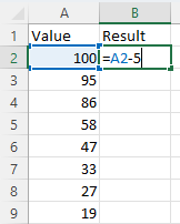
- Select the topmost cell in an empty column to the right of the column with the values you want to subtract from.
- Enter the formula into the blank cell to subtract the number from the topmost cell in the column. For example, “=A1-5”.
- Press enter, and Excel will display the result in the topmost cell of your results column.
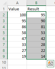
- Drag the fill handle down to extend the operation to the remaining cells in the column. Excel will adjust the cell references appropriately and subtract the number from each cell.

How To Subtract Dates in Excel
Fortunately, it is nearly as easy to subtract dates in Excel as it is in numbers.
This is because, behind the surface, Excel stores dates as sequential serial numbers, which makes them easy to use in calculations.

By default, January 1st, 1900, is stored as number 1 in Excel, and every day past this will always increase the number by 1.
This means that January 7th, 1900, would be stored as seven because it is six days after January 1st, 1900, and correspondingly, January 1st, 2010, would be stored as 40178 because it is 40,177 days after January 1st, 1900.
Fortunately, you don’t need to even think about this or bother counting up all the days since the start of 1900.
Instead, most functions will automatically convert your date values into serial numbers while displaying them in a date format.
All you need to know is that this allows you to effortlessly subtract dates and find the difference.
For example, if you want to find how many days are between two dates, you can subtract them to find out, and Excel will simply subtract the serial numbers in the backend to find out.
Suppose you have a range of start dates and end dates for a series of projects, and you want to know their duration.
All you would need to do is use a simple subtraction formula like you did when subtracting cells like above. For example:
=Cell1-Cell2
Simply substituting in your cell references will allow Excel to take the dates from the cells and subtract them to provide you with the difference in days.
If this fails to produce the expected result, one of the most common causes is that the data contained within the cells are not in a format that Excel recognizes as a date.
This may result from entering dates with periods instead of a slash, such as 01.01.1900.
When this occurs, Excel will be unable to recognize it as a date, and it will instead be formatted as “Text,” which means you will not be able to perform subtraction.
This can be solved simply by re-formatting the text into an ordinary date format that Excel can recognize.
Another issue that may result is that, in some cases, Excel may provide you with a date instead of a number if it uses the format it finds in corresponding columns.
This can be solved simply by selecting the cells and adjusting the format to “General.”
This can be done by navigating to the “Home” tab and choosing “General” from the format drop-down menu. This will convert the result to a number instead of a date.
How To Subtract Time in Excel
Like with dates, it is possible and, in fact, easy to subtract times in Excel because they are stored as numbers below the surface.
While dates are stored as whole numbers, times are stored as decimal values.
This makes sense because if you want to represent a time of day within a specific date, it makes it possible for Excel to store this data in a single number.
For example, if you wanted to represent the time 12:00 pm on January 2nd, 2010, it would be represented by the serial number 40179.5.
This means that when you input time values in Excel, they will be displayed in an ordinary time format but stored as decimal values.
This means that Excel can easily use them in operations. Just as above, you can simply use the ordinary subtraction formula, inputting the appropriate cell references like the following.
=Cell1-Cell2
Or you can put the specific values in as well by substituting your values into the formula:
=TIMEVALUE(“10:00 PM”)–TIMEVALUE(“10:00 AM”)
It is possible that Excel will return the result as a time rather than a numerical value. Using the example in the formula above, it may return 3:00 AM instead of .5. When this happens, it is easily solved simply by converting the result into “General” format using the Drop-down menu.
When subtracting times in Excel, remember that the value will be in decimal value.
You can convert this into hours by multiplying the result by 24.
In turn, the value can be converted into minutes by multiplying by (24*60) and seconds by multiplying it by (24*60*60).
Subtracting Percentages in Excel
Subtracting one percentage value from another can be performed in the same way you would subtract two whole numbers (i.e. =20%-10%).

However, this strategy will not work when subtracting a percentage from a whole number or a decimal.
When you subtract a percentage value, Excel will convert this into a decimal value, run the calculation, and then return it to you as a percentage.
Unfortunately, this results in inaccurate results which is why you will need to follow a slightly different process.
In order to subtract a percentage from a non-percentage value, you can instead multiply by the percentage and then subtract it.
For example, suppose you wanted to subtract 10% from 100 contained in cell A1; you can use this formula:
=A1-(A1-10%)
Conclusion
Excel is an incredibly useful tool for analyzing data and performing operations using it.
Now you know how to use this tool to perform subtraction both between one or more values and cells as well as for dates, times, and percentages.
By understanding how to perform these operations, Excel can be an even more powerful analytical tool.
