An Easy Guide to Square a Number in Excel2 Simple Methods


Finding simplicity and convenience with spreadsheets like Excel has now become easy.
We can now determine squares of numbers at a single point in time, from small to overwhelming numbers.
There are two easy methods to square a number in Excel:
- By a Formula
- By a Function
Don’t worry!
These methods can be done in just a snap and both methods work in the same way.
This tutorial will demonstrate how to use both methods shown above to find the square of a number using Excel.
Squaring a Number in Excel in Two Easy Tricks
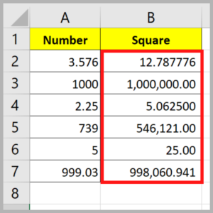
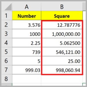
Take a look at the following dataset to understand squaring numbers in Excel quickly:
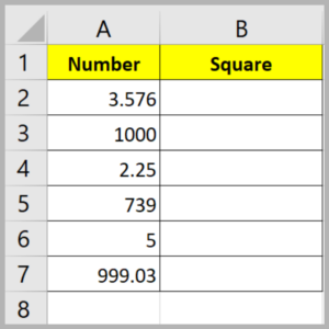
To determine the square of each of the values above shown in column A and the result in column B, let’s take a closer look at how to do this in Excel.
Square a Number by Formula
Squaring a number is very simple.
Just take a number, multiply it by itself or raise it to the power of 2.
Based on the above example, the formula can be written in two ways:
- Multiply it by itself using the multiplication operator
- Raise the number to the power of 2 using the caret operator
Using the Multiplication Operator
In Excel, the arithmetic operator “asterisk” (*) is known as the multiplication symbol.
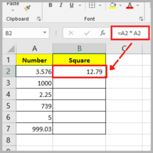
Use the formula to multiply the value in cell A2 by itself using this:
=A2*A2
Accordingly, follow the steps below to determine the square of each number in our given dataset:
- Select the cell you want to display the result (Cell B2).
- Input the formula =A2*A2.
- Press the enter key.
- The result in cell B2 is now the square in A2.

- Drag the fill handle to the last row of your data.
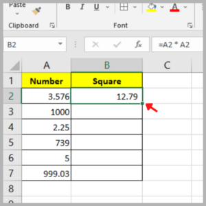
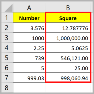
- The square of each value in column A should now be displayed on the corresponding cells in column B.
Using the Caret Operator
The exponentiation operator “caret” (^) is known as the exponent symbol in Excel.
Use the formula below to square the value in cell A2 by raising it to the power of 2:
=A2^2
Accordingly, follow the steps below to determine the square of each number based on the dataset given:
- Select where you wish to display the result (Cell B2).
- Type the formula =A2^2.
- Press the enter key.
- The result in cell B2 will show the square of the value in A2.

- Drag the fill handle down to the last row of your data.
- The square of each value in column A should now be displayed on the corresponding cells in column B.
Using a Power Function to Square a Number
Raising a number to a specific power is also one of Excel’s useful functions.
The POWER function works just like the exponent used in a math equation and raises one number to the power of another number.
The syntax used for the POWER function is shown below:
=POWER(number,power)
Where:
- Number = corresponds to the number that you wish to raise to an exponent.
- Power = the exponent you wish to raise the number to the power of.
Therefore, to find the square of a number using the POWER function, you have to raise it to the power of 2 as shown below:
=POWER(A2,2)
Accordingly, follow the following steps below to determine the square of each number based on the given data:
- Select the cell you want to display the result (Cell B2).
- Type the formula =POWER(A2,2).
- Press the enter key.
- The result in cell B2 is now the square of the value taken from A2.

- Drag the fill handle down to the last row of your data.
- The square of each value in column A should now be displayed on the corresponding cells in column B.
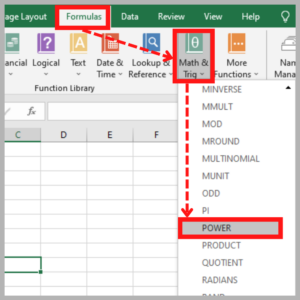
Note: The POWER function can be found in the Formulas tab with the Math & Trig functions (under Function Library).
It should be below the Select a Category drop-down list if you’re in the Insert Function dialog box.
This tutorial has demonstrated how to use the above methods to find the square of a number in Excel using three easy and quick methods.