How To Split Cells in Excel (separate into multiple columns)Step by Step Instructions with Screenshots

Last Updated: February 9, 2023

When using Excel, particularly in cases where you are working with imported data, it is extremely common to come across multiple pieces of information located in the same cell.

When this occurs, you often may find that you need this data separated into its individual components.

This issue often arises when you need to present data in a different form than its original authors.

Regardless of the reasons, when this issue arises, you need to separate the data located in one or more cells into multiple columns.

Fortunately, Excel provides multiple relative ways to do this.

Depending on the specific data you need to separate and its consistency, some methods may work better than others.

Let’s take a look at some of the easiest and most effective ways.

Split Cells into Multiple Columns with the Text to Columns Wizard

Perhaps the easiest way to split the components of cells into multiple columns is using a little-known built-in feature in Excel.

This is the “Text to Columns” feature which is located right on the ribbon and uses either fixed character lengths or delimiters such as spaces, hyphens, or commas to determine where to separate data in your cells.

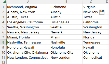
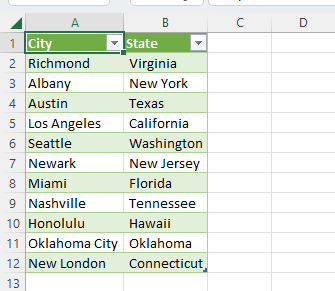
As an example, consider a series of cities and states located in one column, and you want to separate the names of each state into a second column.

To do this using the Text to Columns feature, follow the steps below.

Select each of the cells containing data you want to split into multiple columns.

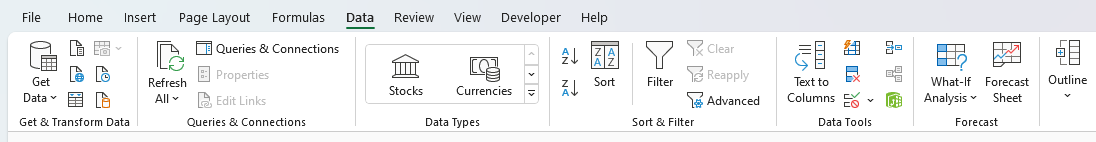
On the ribbon, navigate to the “Data” tab, and in the “Data Tools” group, select “Text to Columns.”

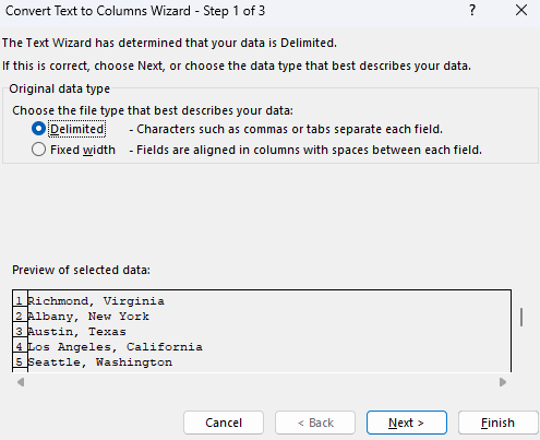
This will open the “Convert Text to Columns Wizard,” which you will use to separate the text in your cells.
On the first screen, under the “Original data type” selection, choose “Delimited.” This will allow you to separate the data using the occurrence of certain characters, which in this case will be the comma occurring after each city. This will, of course, be different for many data sets and may instead be a hyphen or even a space. Once selected, press “Next.”

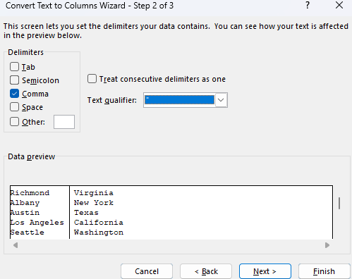
In the next window, you will enter the specific delimiter for your data. In this case, you will place a check in the “Comma” box and then select “Next” to continue.

In the last step, the “Text to Columns Wizard” will ask how you want the results to be formatted and placed in the worksheet. Since the data is simply text, the “General” or “Text” format will be fine, and for the destination, the column located right next to the existing data will be fine. Once completed, select “Finish.”

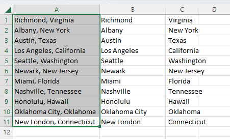
That is all there is to it, and now the data is neatly separated into multiple columns.

It is hard to get easier than that, but there are a few drawbacks to this process.

First of all, this is not a dynamic feature meaning that the resulting cells will not be updated when changes occur in the source data.

When this occurs, you will need to go through the entire process using the “Text to Columns Wizard” again.

A second issue is that the “Text to Columns” feature does not work well unless the data in each cell is in a uniform format with either consistent delimiters or length, which Excel can use to determine where to split the data.

For example, if part of the data used one hyphen and other parts used two, the Wizard may not be able to produce consistent results.

Split Cells into Multiple Columns with Flash Fill

Chances are, if you are using any version of Excel starting from Excel 2013, you have used Flash Fill, possibly without even thinking of it.

This incredible feature makes it possible for you to split cells without using any complicated formulas or menus.

So, long as your data has consistent patterns that Excel can use to determine what it is you want to do, you can separate cells instantly, and here is how.

In the columns next to your source cells, enter a few examples of how you would like your data to be extracted. For instance, enter a few of the cities and states into their respective columns. This will give Excel an example of the pattern it should follow in extracting the data.

If, at any point in entering the data, Excel displays your text in the cells in the way you would like it to be separated, you can simply drag the fill handle down or press “Tab” to let Flash Fill extract your text. Often this will happen after manually extracting data into the second row in a given column.

If this does not occur, you can try executing Flash Fill manually instead. After entering data into a few cells, select all of the cells in the range you want Excel to extract the values.

Navigate to the “Home” tab, and under the “Editing” group, select “Fill.” This will open a drop-down menu where you can select “Flash Fill,” which will automatically enter your data into the selected range.

While Excel’s Flash Fill feature is good at detecting patterns in data in order to auto-complete repetitive tasks like separating data into multiple columns, it is not perfect. In more complex data sets, it is quite possible that they will not return the correct values.

Flash Fill may, in some cases, be unable to detect a pattern that it can follow at all. If this occurs, then Excel will display an error message stating that it was unable to detect a pattern for filling in values.

Finally, like with the Text to Columns feature, Flash Fill is not dynamic and thus will not update with changes in the source cells. You will instead need to rerun the process when changes occur.

Split Cells into Multiple Columns with Power Query

Power Query is another option for splitting data in a cell into multiple, and it has been available as a built-in option in versions since Excel 2016 and as an add-on for the 2010 and 2013 versions.

The Power Query editor is a powerful tool that can split cells and columns with ease.

This may not be as easy to use as the previous two options, but it has several advantages, as you will soon see. Simply follow the steps below to get started.

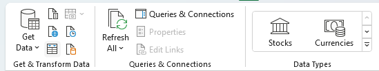
First of all, select any of the cells in your data set and navigate to the “Data” tab. Within the “Get & Transform Data” group, select the “From Table/Range.”
If your data is not already in a table, this will prompt Excel to open the “Create Table Dialog box. Ensure that the entire range of data is selected, check the box next to “My table has headers,” and then click “OK,” This will open the “Power Query Editor.”

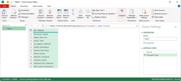
With the “Power Query Editor,” it will display a preview of the selected data, which you can use to confirm that the table Excel has created contains your raw data.
Using the ribbon of the “Power Query Editor,” navigate to the “Home” tab and select “Split Column” from the “Transform” group. On the drop-down list that appears, you can choose from a wide range of options that can be used to separate the contents of the selected cells. However, for our current example, we will be using “By Delimiter.”

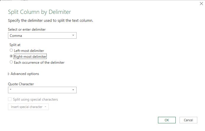
This will open the Split Column by Delimiter” menu, where you can set the parameters for how your data will be split. There are many options to use depending on how the contents of the cell are formatted and where the delimiter occurs within the data. However, in our case, we simply need to select “Comma” in the “Select or enter delimiter” box, and any of the options for “Split at” will work, so we selected “Right-most delimiter.” Once everything is selected, press “OK.”

The data preview window will now update and show how the cells have been split according to the setting you chose. Ensure that they look correct and then update the column headers appropriately, for instance, “City” and “State.” Simply double-click the column headers to rename them, and while you are at it, you can perform many other transformations to file and sort data while you are in the editor, so take your time to explore.

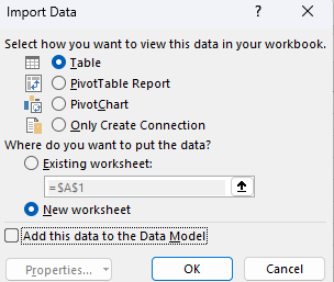
When you are done making changes to your data, it is time to get it back in Excel, and to do this, navigate to the “Home” tab and select “Close & Load.” This will open a drop-down menu where you can choose to load your data into a new or existing worksheet. In order to place your data into a new worksheet, simply select “Close & Load.” If you would prefer to have the data placed in a particular location, for example, next to the source cells, click “Close & Load to…” and select the worksheet and cell references on the “Import Data” dialog box and click “OK.”

When you are finished, the now separated cells will now be loaded back into Excel.

The Power Query editor is not the fastest way to separate cells, but it is a bit more flexible in its ability to separate cells than the above options.

Power Query can not depend on delimiters to separate cells and can potentially handle more complex data by using “Column from Examples.”

Also, one of its best features is its ability to update. If the data in source cells change or if more data is added, it is as easy to update as navigating to the “Data” tab and selecting “Refresh All.”

This is not fully dynamic; however, it is relatively easy to do and prevents having to run through the full procedure again.

The biggest downside to using Power Query is that it can only be used by converting your cells into a table which may not always be an option depending on the situation and data source.

Fortunately, there is one more easy option for splitting your data that does not depend on delimiters and is fully dynamic.

Split Cells into Multiple Columns with Text Functions

Excel offers many different text functions for manipulating text strings, and a few of them can accomplish splitting a cell into multiple columns.

Unlike other options, there are no firm rules to follow in order to split your cells; instead, you can use any rules that you can program into a formula.

This is incredibly powerful and means there are virtually no limitations to what you can do, but it also requires a lot more skill with no simple interface to work with.

Though Excel offers many different text functions, the most important ones for our uses are:

LEN: Provides the length of a string;
LEFT: Extracts a given number of characters out of a string’s left-most end;
RIGHT: Extracts a given number of characters out of a string’s right-most end;
MID: Extracts a substring from a specified position within a string; and
Search: Determines the position of a substring in a string.

There is no fixed way to use these functions, and they can, in fact, be used in any combination to split cells based on the particular situation and text strings.

However, we will look at an example of how to use these tools to accomplish a simple extraction.

To separate our city and state example using these tools, we will use a combination of the LEFT, RIGHT, LEN, and SEARCH functions. Here is how:

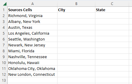
Determine how you want to split the data. In our example, we will continue using the cities and states, which means that the data we want to split is separated by a comma. We also want to place the data in the two columns to the right of the source cells, so we will prepare them with headers.

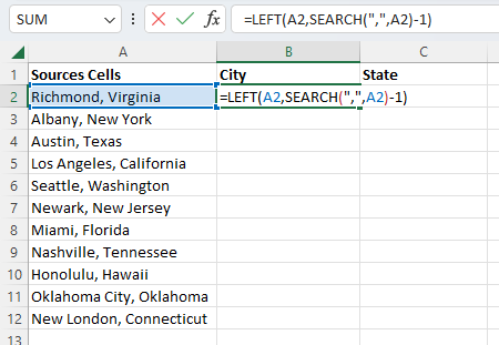
In the cell to the right of our first source cell, we will enter the formula =LEFT(A2,SEARCH(“,”,A2)-1). In this formula, the SEARCH function will look for any comma in the text string and return its position. Since we don’t want to include the comma in the resulting cell, we subtract one, and then the LEFT function will extract the resulting number of characters from the left side. Excel will then display our resulting string.

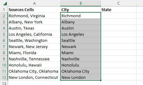
Though we could copy and paste the formula into the remaining rows while manually adjusting the cell references in order to extract the cities we need, this could be time-consuming. Fortunately, we can extend our formula to the remaining rows much easier by selecting the fill handle on the bottom-right of the cell and dragging it down as far as we need, and Excel will run the same formula in each cell, giving us all of our cities.

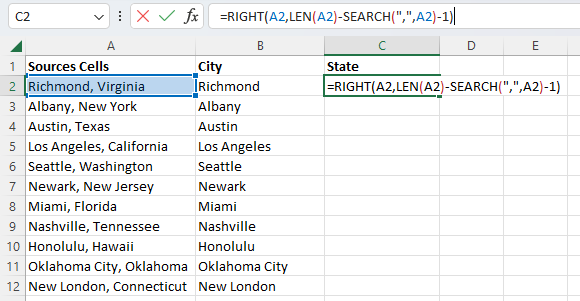
Now we need to separate the other part of our cell into the next column, and to do this, we can follow a similar process, but we will instead need to use the RIGHT function to extract the substring from the other side of the cell and account for the additional space after the comma. We will enter the formula =RIGHT(A2,LEN(A2)-SEARCH(“,”,A2)-1); press “Enter” on our keyboard, and Excel will extract the state and display it within the cell.

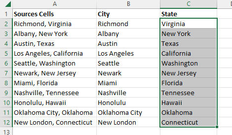
Now, in the same way, as for extracting the first part of our text, the formula can be copied into the remaining rows with adjusted cell references, or the fill handle can be used to automatically extend the formula into the remaining cells. Regardless of which method is chosen, the result will be the same.

It is clear that text functions require a bit more skill and time investment than the previous methods, and depending upon the complexity and consistency of the text strings that need to be split, the formulas can become extremely complex.

However, unlike previous methods, there are few limitations to what can be accomplished with text formulas.

In addition, text formulas are the only truly dynamic option among these ways to split cells.

This means that whenever the source cells change, the resulting cells will automatically update as well.

This can be extremely useful when the source data continue to be updated regularly.

Conclusion

Now you have seen four different techniques you can use to separate cells into multiple columns in Excel.

This includes using Text to Columns, Flash Fill, Power Query, and text functions.

Each of these methods can work and has its own advantages ranging from extreme simplicity to being flexible and able to handle more tasks.

It is best to familiarize yourself with each of these options and choose the one that is best suited to your situation.