Utilizing Slicers in Excel for Charts and Pivot TablesTutorial with Screenshots and More!

Last Updated: February 22, 2023

In this tutorial, we will demonstrate how to incorporate slicers into tables, pivot charts, and pivot tables in Excel.

Furthermore, we will delve into more advanced techniques, such as customizing slicer styles, linking a single slicer to numerous pivot tables, etc.

One of the most robust tools for creating summary reports and summarizing massive volumes of data is the Excel Pivot Table.

You can create your reports more interactive and user-friendly by including visual filters, also known as slicers.

You also have the option to give your coworkers access to your pivot table with slicers, so they won’t have to bother you every time they need the data to be filtered in a different way.

Excel Slicer

Excel slicers are pivot tables, tables, and pivot charts that can all be filtered graphically. They complement summary reports and dashboards with their graphical qualities but can be used in any scenario to streamline data filtering processes.

Slicers were first introduced in Excel 2010 and can be utilized in Excel 2013, 2016, 2019, and later versions.

Here’s the step-by-step process for filtering pivot table data using one or multiple buttons in the slicer box:

Comparing Excel Slicers and PivotTable Filters

Pivot table filtering can be cumbersome, but with slicers, it is as easy as a single button click.
Slicers can be attached to numerous pivot tables and charts, however, filters can only be connected to one pivot table.
Filters are confined to columns and rows, but slicers are flexible objects that can be positioned anywhere, even inside the area of the chart for real-time updates on a touch.
Slicers perform better in many touchscreen contexts than pivot table filters, except for Excel mobile.
Slicers use more worksheet space than pivot table report filters, which are more compact.
Automating pivot table filters with VBA is straightforward, but slicer automation will require more technical know-how.

Instructions on Adding a Slicer in Excel

To begin using slicers, follow these guidelines for adding a slicer to your Excel Pivot Table, Table, or PivotChart.

Instructions for Adding a Slicer Excel Pivot Table

It is quick and simple to add a slicer in Excel Pivot Table. Simply follow the steps outlined below:

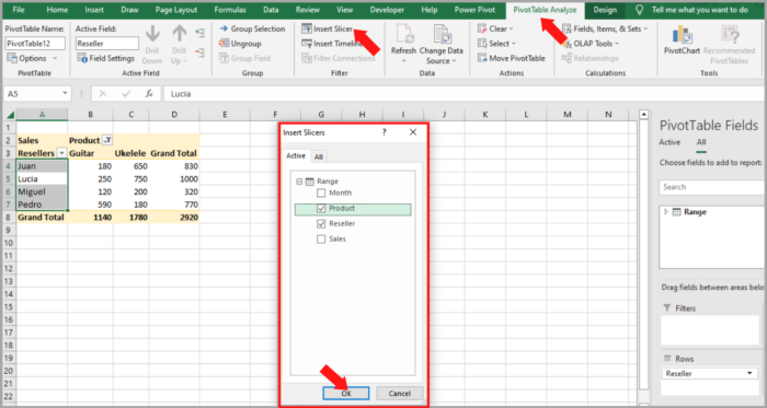
Select anywhere within the pivot table.
In Excel 2013, 2016, and 2019, navigate to the Analyze tab > Filter group and proceed to click on Insert Slicer. For Excel 2010, go to the Options tab and choose Insert Slicer.
A dialog box named Insert Slicers will appear showcasing checkboxes for each pivot table field. Pick one or multiple fields to add a slicer to.
Confirm by clicking OK.

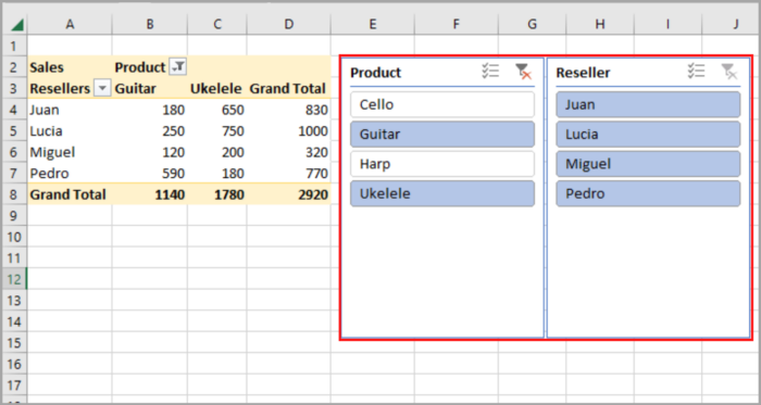
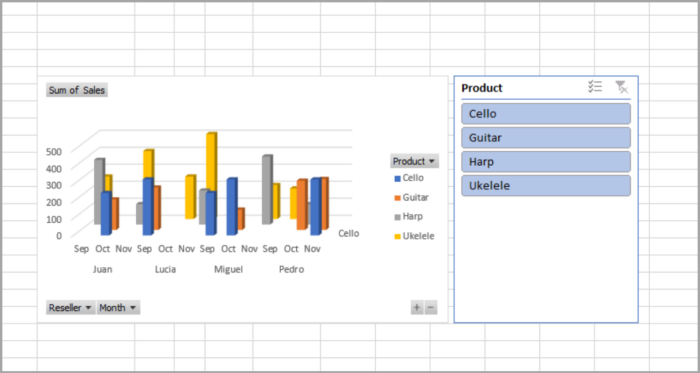
For demonstration purposes, let’s create two slicers to filter the pivot table based on Reseller and Product.

Instantaneously, two slicers for the pivot table will be established.

Creating an Excel Table Slicer

Excel 2013, 2016, and 2019 also offer the option of adding a slicer to a standard Excel table. The process is as follows:

Select any cell within the table.
Go to the Insert tab -> Filters group -> Slicer.
Choose the desired columns to filter in the Insert Slicers dialog box.
Finally, click OK to insert the slicer.

With just a few clicks, you can now take advantage of the visual filter provided by the Excel slicer to easily sort through your data table.

Adding a Slicer to a Pivot Chart in Excel

You can simply create a slicer for the pivot table as explained in the section above and use a slicer to filter a pivot chart.

The slicer will then control the pivot chart as well as the pivot table.

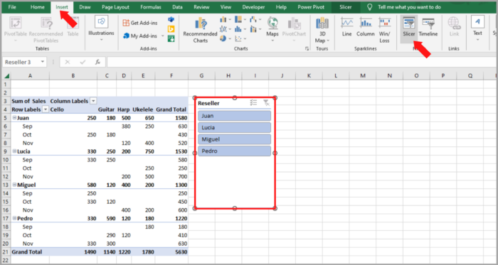
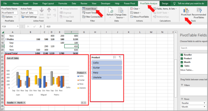
To create a slicer for a pivot chart that controls both the chart and the pivot table, follow the following steps:

Click on any cell within your chart.
Navigate to the Analyze -> Filter group and proceed to the “Insert Slicer” button.
In the “Insert Slicers” dialog, choose the fields you wish to add as slicers and hit “OK”.

Your worksheet will now have a slicer box.

To use the slicer to filter the data of your pivot chart, you simply have to click on the desired filter option in the slicer box.

As an improvement, you can make the chart’s filter buttons become invisible because they will no longer be needed since the slicer is now doing the filtering.

Moving the slicer box inside the chart area is another change you may do. You can achieve this by sliding the borders to make the plot area smaller and the chart area larger.

The slicer box can then be dragged to the empty area that has just been created.

Here’s a tip: Right-click the slicer and choose “Bring to Front” from the context menu if it becomes obscured behind the chart.

Using Slicer in Excel

With the easy-to-use design of Excel slicers, filtering your data has never been simpler.

This section will provide you with some tips to help you get started.

Utilizing Slicers as a User-Friendly Filter for Pivot Tables

With a slicer set up for a pivot table, filtering your data is as easy as clicking the desired buttons in the slicer box.

The pivot table will instantly reflect the updated data based on your selections.

If you need to delete a filter, deselect the item, and click the relevant button in the slicer.

Using a slicer, it’s possible to filter information that is not available in the pivot table.

For instance, by inserting a Product slicer, the slicer can still be utilized to filter the pivot table by product, even if the Product field is hidden.

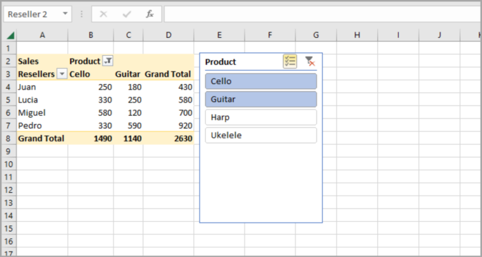
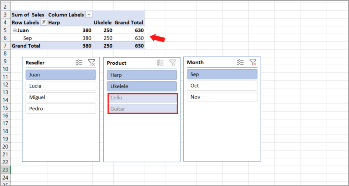
If you have multiple slicers linked to a similar pivot table and you select a specific item in one slicer, some options in the other slicer may become greyed out, indicating that there is no data available for that combination.

As an illustration, if you choose “Juan” in the Reseller slicer, “Cello & Guitar” in the Product slicer will turn gray, signaling that Juan did not sell any “Cello & Guitar”.

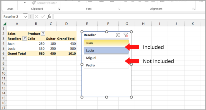
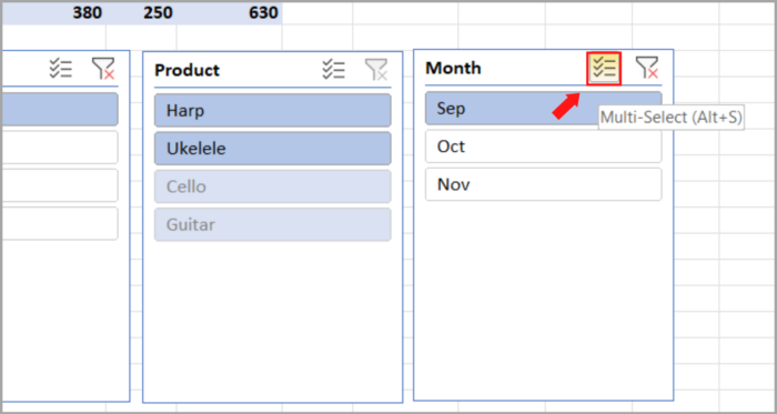
Techniques for Selecting Multiple Entries in a Slicer

Three methods exist to pick more than one item:

Hold down Ctrl and click the slicer buttons.
Activate Multi-Select by clicking it (as shown in the screenshot), and then individually select items.
Click within the slicer box, hold down Alt + S to enable Multi-Select mode, choose the items, and finally hold down Alt + S again to turn off Multi-Select.

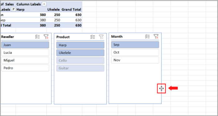
Relocating a Slicer in Excel

To relocate a slicer in an Excel worksheet, drag it to a different spot by moving your mouse over it until the cursor changes to a four-pointed arrow.

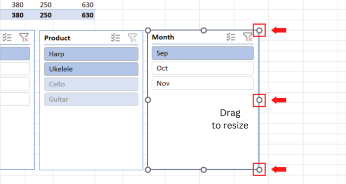
Resizing Slicer

Changing the size of a slicer in Excel can be done by two methods: (1) by dragging the box’s edges, or (2) by selecting the slicer and adjusting the width and height in the “Slicer Tools Options” tab.

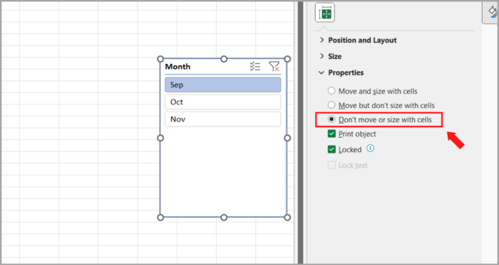
Locking the Position of a Slicer in the Worksheet

Making a slicer stay in a specific position in a worksheet will require these steps:

Right-click on the slicer then select “Size and Properties.”
Under the pane “Format Slicer, right under Properties, check the box that says “Don’t move or size with cells.”

This ensures that the position of your slicer remains the same even if you make changes to the sheet like adding or deleting rows and columns or adding or removing pivot table fields.

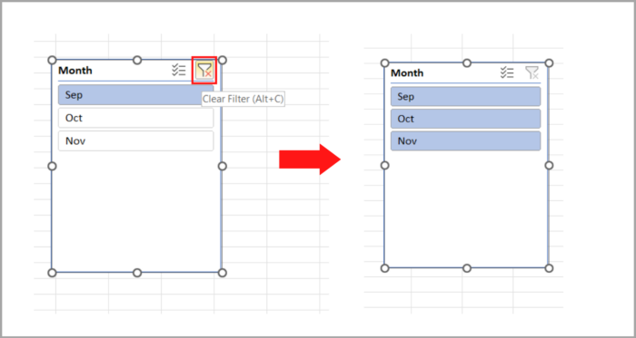
Removing a Slicer Filter

To clear the filter in an Excel slicer, you can use any of the following methods:

Hold down Alt + C keyboard shortcut while clicking anywhere in the slicer box.
In the top right corner, click the button “Clear Filter”.

This action will result in all items in the slicer being selected, effectively removing the filter applied by the slicer.

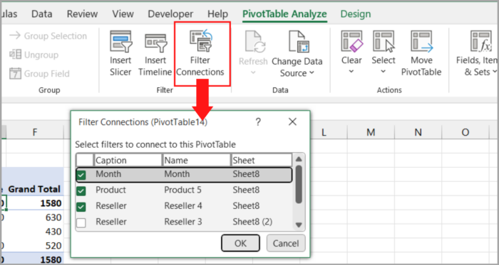
Removing a Slicer’s Connection to a Pivot Table

To break the connection between a slicer and a specific pivot table, the following steps should be taken:

Decide which pivot table you want to remove the slicer from.
Go to the Analyze tab > Filter group, then select Filter Connections (this is applicable for Excel 2019, 2016, and 2013). In Excel 2010, select Insert Slicer > Slicer Connections on the Options tab.
Uncheck the box next to the slicer you wish to disconnect in the Filter Connections dialog box.

It’s important to note that disconnecting a slicer from a pivot table won’t remove the slicer itself from your worksheet.

Open the Filter Connections dialog box once more and choose the slicer if you want to reestablish the connection later.

When the same slicer is connected to many pivot tables, this strategy might be useful.

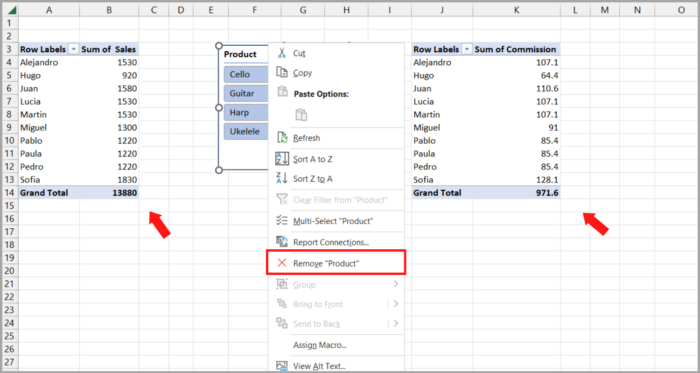
Removing a Slicer in Excel

One of the following actions can remove a slicer from your worksheet permanently:

Press the Delete key while selecting the slicer.
Click Remove <Slicer Name> after you right-click on the slicer.

Customizing Excel Slicers

Customizing Excel slicers is simple and can be done by altering their appearance, colors, and configurations.

This article will explore how to refine the default slicer created by Microsoft Excel.

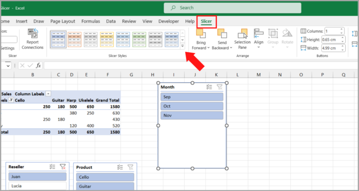
Altering the Style of a Slicer in Excel

To modify the appearance of a Slicer in Excel, follow these steps:

To make the tab of the Slicer Tools show on the ribbon, select the slicer.
Under the tab Slicer Tools Options, choose the desired style thumbnail.

Note: Select the More button to view the full range of slicer designs.

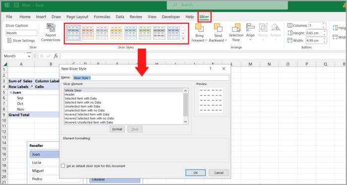
Creating a Personalized Excel Slicer Style

To create a custom slicer style in Excel, follow these steps:

Click “More” when you click on the tab “Slicer Tools Options” -> Slicer Styles group.
At the foot of the Slicer Styles collection, click the button “New Slicer Style”.
Give a name to your new slicer style.
Select the options for formatting for each element of the slicer.
Click OK to save the custom style and make it available under the Slicer Styles gallery.

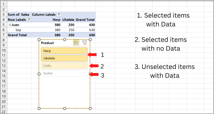
To help you understand the various slicer elements, here’s a breakdown:

Slicer pieces marked “With Data” are connected to specific data in the pivot table.
Slicer items that include “With no Data” attributes indicate that the pivot table has no data (e.g. the source data was removed after the slicer was created).

Note:

To create a unique slicer design, select the built-in style that resembles your desired design and make a copy of it. Then, modify the elements to suit your needs and save the new style under an alternative name.
To make your custom slicer styles available in future workbooks, the workbook has to be saved containing the styles as an Excel Template file (*.xltx). New workbooks created from this template will include the custom slicer styles.

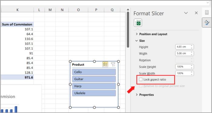
Using Several Columns in an Excel Slicer

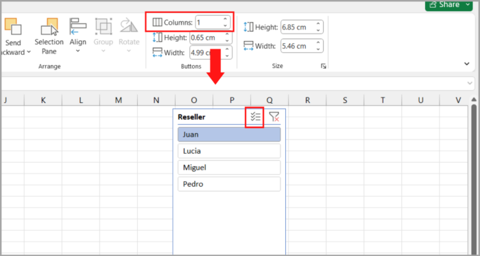
To display many slicer items without scrolling, arrange them into multiple columns:

Select the slicer and proceed to the Slicer Tools Options tab to access the Buttons group.
Enter the desired number of columns in the Columns box.
Change the slicer box’s and the buttons’ height and width if necessary.

This will give you a clearer view of the slicer items without the need to move up or down.

Behind the pivot table, this method can be used to give your slicer a tabbed appearance:

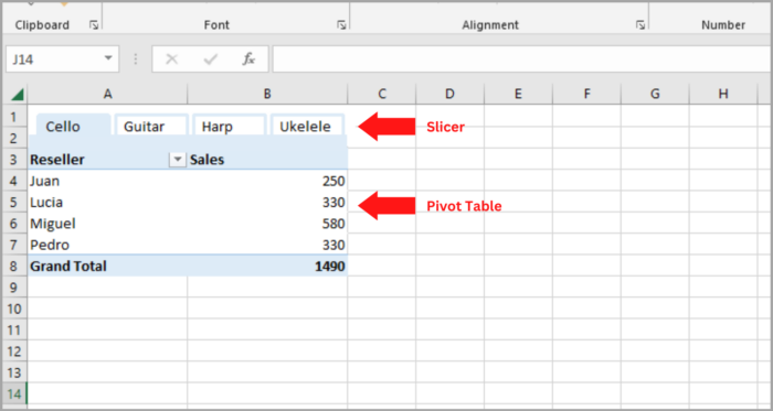
Follow the modifications to be made to the slicer to create the illusion of tabs using the information below:

Arrange the slicer in 4 columns.
The header of the slicer was hidden (refer to the instructions).
A custom style was created, in which the slicer’s border was removed and the fill color of the “Item with data selected” was changed to match the header row’s color in the pivot table. Consult the “How to build a custom slicer style” tutorial for further details.

Changing the Setting of the Slicer

The beauty of Excel slicers lies in the fact that they can be tailored to your exact specifications. Right-click on the slicer and select “Slicer Settings…” and a dialog box will appear displaying the default options (as shown in the accompanying screenshot).

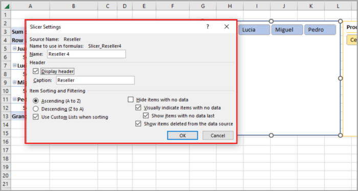
The Slicer Settings dialog box provides a range of customizations to enhance your slicer’s functionality. Some notable options include:

Clear the Display header option to make the slicer header invisible.
Arranging slicer items in ascending or descending order.
Concealing items without data by unticking the relevant box.
Preventing the display of deleted items from the source data by unchecking the related checkbox. This ensures your slicer only shows up-to-date information.

Linking a Slicer to Several Pivot Tables

To create robust cross-filtered Excel reports, consider utilizing a slicer that connects to multiple pivot tables.

Fortunately, this capability is offered by Microsoft Excel and is relatively straightforward to implement. Here’s how:

Generate several pivot tables within the same sheet, if possible.
For easy identification, give descriptive names to each pivot table. Enter a name in the PivotTable Name box in the top left corner of the Analyze tab.
As usual, make a slicer for any pivot table.
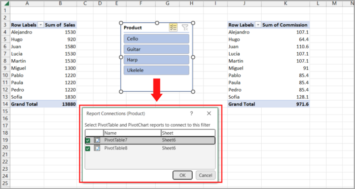
Right-click the slicer then select “Report Connections” (or “PivotTable Connections” in Excel 2010). Another option is to choose the slicer, go to the “Slicer Tools Options” tab, choose the “Slicer” group, and then press the “Report Connections” button.
Select every pivot table you want to link to the slicer in the Report Connections dialog box, then click OK.

Going forward, you can easily filter all linked pivot tables with just one click on the slicer button.

Similarly, it is possible to associate a single slicer with several pivot charts.

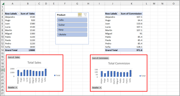
Important Note: Only pivot tables and charts that use the same data source as the slicer can be attached.

Unlocking Slicer in a Protected Worksheet

If you want to restrict the editing of pivot tables but still allow users to select slicers when sharing your worksheets, follow these steps:

Hold down the Ctrl key while selecting the slicers to unlock them all at once.
Select “Size and Properties” from the shortcut menu by right-clicking any of the selected slicers.
Uncheck the “Locked” option in the “Properties” section of the “Format Slicer” panel, then close it.
Click Protect Sheet in the Protect group under the Review tab.
Tick the Use PivotTable & PivotChart box in the Protect Sheet dialog.
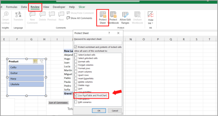
As an optional step, type a password and press OK.

With this configuration, you may now share your spreadsheets without worrying about the security of your data even with beginner Excel users.

They will continue to be able to use the dynamic reports with slicers even if they are not able to change the layout and structure of your pivot tables.

I hope this guide provided valuable information on how to add and utilize slicers in Excel.