How to Separate Names in Excel Five Easy Methods!
In Excel, when you separate full names into columns, it is easier to perform any of the Excel operations such as Search, Sort, Filter, etc.
Separating names is commonly used in data processing tasks. Excel should have a dedicated function for it.
Nonetheless, there are many ways in which you can separate names in Excel.
This tutorial will show you how to do this in 5 easy ways:
- Text-to-Column Feature
- Flash Fill feature (2013 Excel version onwards)
- Find and With (wildcard characters)
- Formula
- Power Query
Separating or Splitting Names in Microsoft Excel
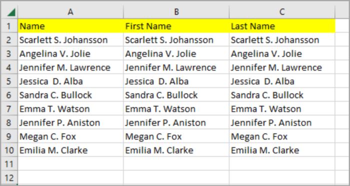
To show you the different methods, let us consider the following list of names as the basis of our example:
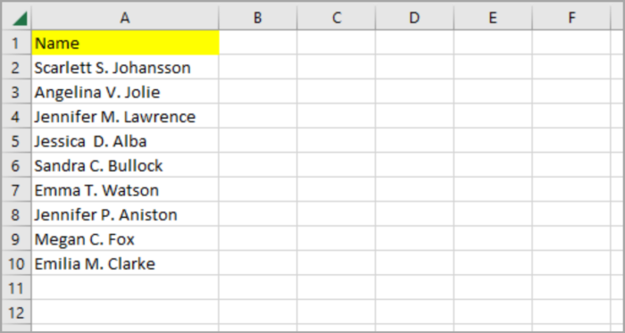
Here you notice all the names contain a middle initial which can be a challenge to extract.
In this tutorial, we will provide you with easy and reliable steps to do this job.
Method 1: Use the Text-to-column Feature to Separate Names in Excel
This method is the most common and easiest way because splitting the name is quick and simple, and we can work with middle names.
However, this works in different naming formats as long as the cell contains a delimiter (comma or space).
Here is the step-by-step process for using this method:
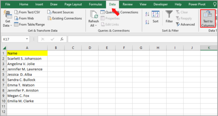
- Click and select the cell range that you want to work with (cells A2:A7).
- Go to the ‘Data menu’. Under the ‘Data Tools’, click ‘Text to Columns’.

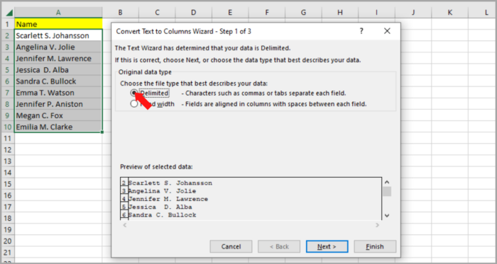
- ‘Convert text to Columns Wizard’ will now appear on your screen.
- The Wizards’ step 1 will let you select how your column is going to be separated – fixed width or by a delimiter. The delimiter that is commonly used is space or a comma, which is why we are selecting the ‘delimited’ option.

- Click the ‘Next button.
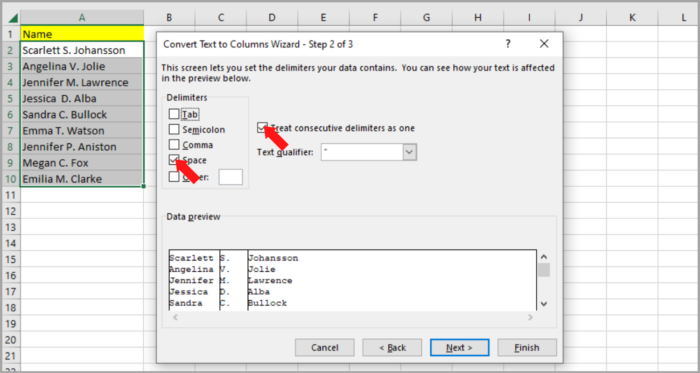
- The Wizards’ step 2 will let you select the delimiter you want to separate the names in your spreadsheet. Check the box beside the’ Space’ if the name is separated by a space.
- Sometimes, users tend to make mistakes entering space. They enter 2 spaces between the names. Excel has a feature that cuts these spaces and considers them as one. By checking the box next to ‘Treat consecutive delimiters’.

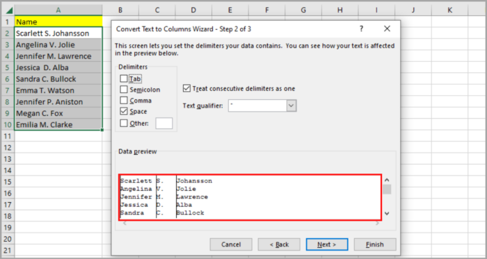
- The bottom part of the wizard lets you see the preview of your work and see the look of your data after the split.

- Click the ‘Next button’.
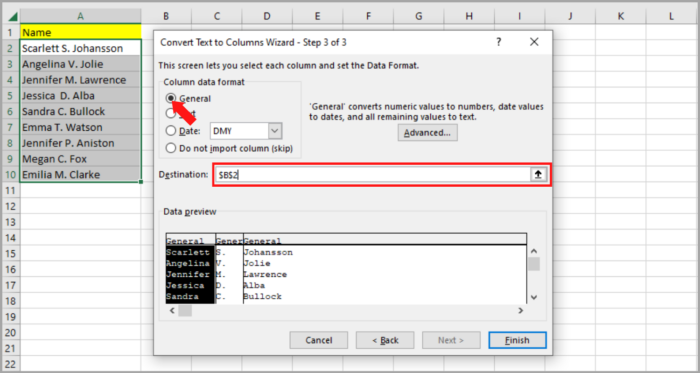
- The Wizards’ step 3 will let you choose the format of each extracted column. Assuming the names are all text, the General option should be selected.
- This format will let you choose where you want the names to be in your separated columns to start. Here we want the original names to remain and separate the names in a new column, let us now declare the cell reference $B$2 in this field.

- Click the ‘Finish’ button.
Now, the names are separated into three columns, one column for the first, middle, and last names. You now have the option to rename each column as ‘First Name’, ‘Middle Initial’, and ‘Last Name’.
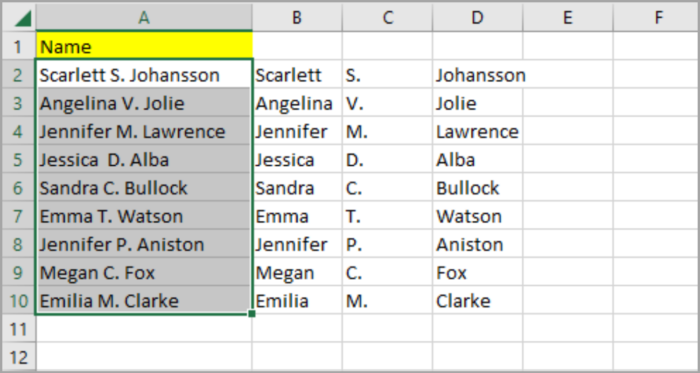
Note: This only works in a consistent format name. For example, all given name has first names, middle initials, and last names. However, if the names are not the same in format, this method will not work.
Method 2: Use Flash Fill Feature to Separate Names in Excel (2013 Version Onwards)
Using Flash Fill is one of the fastest ways in finishing your work if you’re using Excel 2013 version and Up.
Usually, names have a uniform format, and this makes the Flash Fill feature great for separating names into different columns.
Here is the step-by-step process:
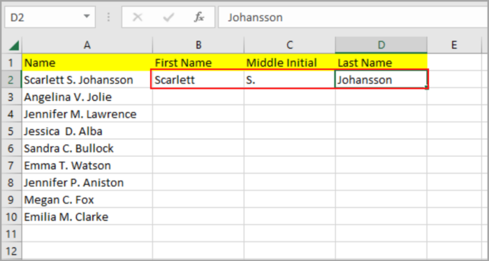
- Manually type the first name located in cell A2 into three separate columns shown in the image below:

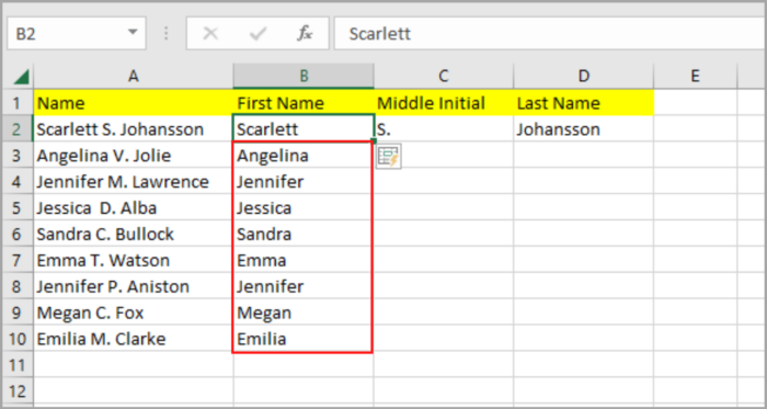
- In the first name column, click on the 2nd row and press the Flash Fill button. You can find the button in the Data tab (under Data Tools). Or you can use the keyboard shortcut CRTL+E for automatic flash fill.

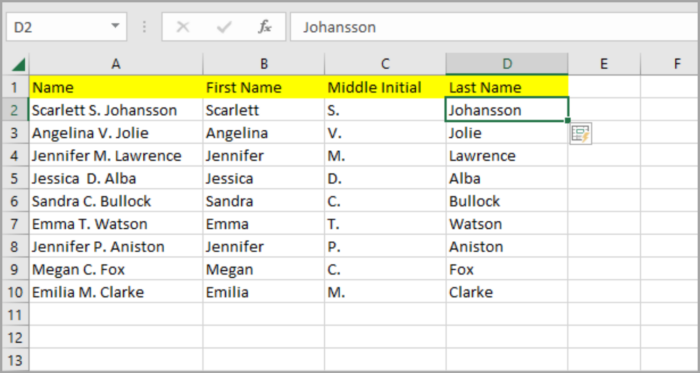
- Repeat Step 2 for the middle initial and last name. Now you can see the names in separate columns.

The Flash Fill feature is great for recognizing patterns, and a great way to separate names even with comma-separated names. Check the image below:
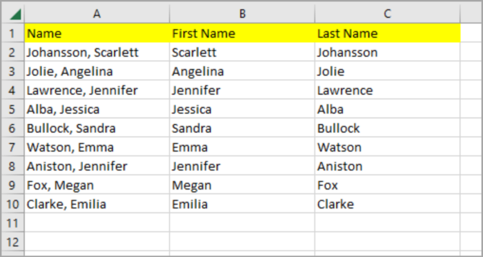
Even when you have a mix of names (with or without the middle name), the flash fill method still works, unlike the Text Column method.
The flash fill feature recognizes the pattern and easily recognizes the first name and the last name in a column.
Note: Make sure that the names are in a uniform format. There would be a time the Flash Fill feature does not work and will give you the wrong results.
Method 3: Use the Find and Replace (wildcard characters)
The Find and Replace feature in Excel is considered a versatile feature since it can do more than just that – it uses wild cards to target specific patterns in your data.
A wildcard is a symbol that represents a set of characters. For example, the asterisk symbol commonly represents numbers or a string of numbers.
If you are looking for all names that start with the letter ‘B’, then you can use ‘B*’ as the string search.
You can extract the rest of the characters that follow a delimiter by combining the asterisk wildcard with the Find and Replace feature like a comma or space character.
The downside is that this method only works in extracting the first and last names. You cannot use it in middle names.
Here is the step-by-step process:
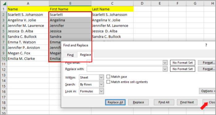
- First, you have to copy the cells that contain the name. Then, paste it into two different columns (for the first and last names as shown in the image below).

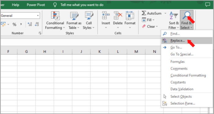
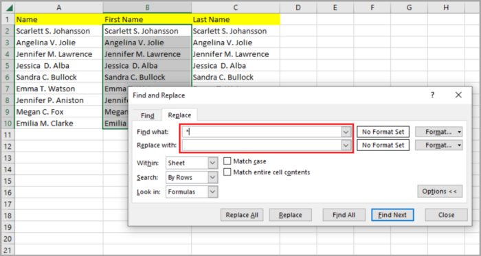
- Click and select the names in the First Name column. Go to the Home tab and click on the Find and Select button (Editing group). A drop-down menu will appear, select the Replace option. The Find and Replace dialog box will appear. You can use the keyboard shortcut CTRL+H as another option.

- Type your search string in ‘Find what’. Type the search string ‘ *’ for the First Name Column (this is a Space character followed by an asterisk symbol).
- In the ‘Replace with’, leave it blank because you want to delete everything after the first name (to be able to extract the first name).

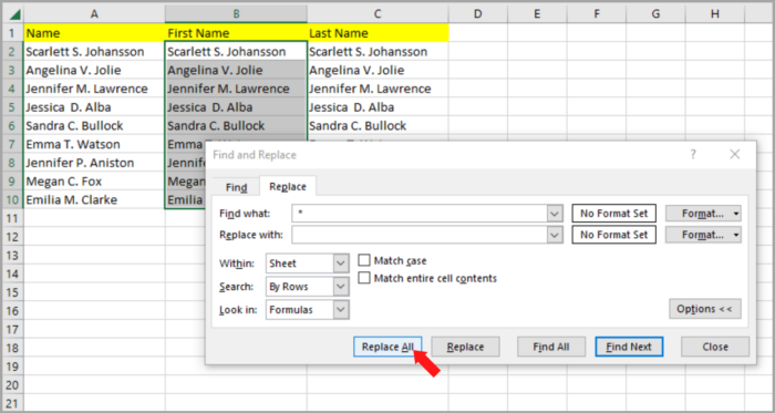
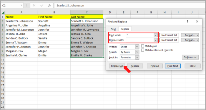
- Click the Replace All button.

- There will be a message box that will appear. This will let you know how many were replaced and now the column contains the first name only.

- Repeat this step 3 to 6 for the Last Name column (except step 4). In the ‘Find what’ search string that we should enter is ‘* ‘ (asterisk symbol, then followed by a space character).

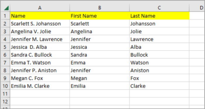
- This should be the finished look of the table. Shown in the image below:

Method 4: Use Power Query to Separate Names in Excel
This method is more complicated than the other methods that we discussed earlier.
But in the long run, this method is more reliable than the other methods, especially if you are using Power Query as part of your data processing toolkit.
You can use this in your Power Query cleaning process and avoid redundancy every time you work with names.
A lot of Excel users are not familiar with Power Query – it is a tool that extracts and transforms data.
This is available in the 2016 Excel version and onwards (located in the Data tab). In the older version, you need to install it as an add-in.
The Power Query has a feature that is data splitting similar to the Text to Columns feature.
In this part of the tutorial, we will show you how this works in splitting names in Excel:
Note: To apply Power Query, your data needs to be in an Excel Table format. To convert your data to an Excel table, just go to Insert>Table. Or you can use the keyboard shortcut CRTL+T. Make sure that it shows the correct range of cell that contains data when creating a table. Lastly, click the OK button.
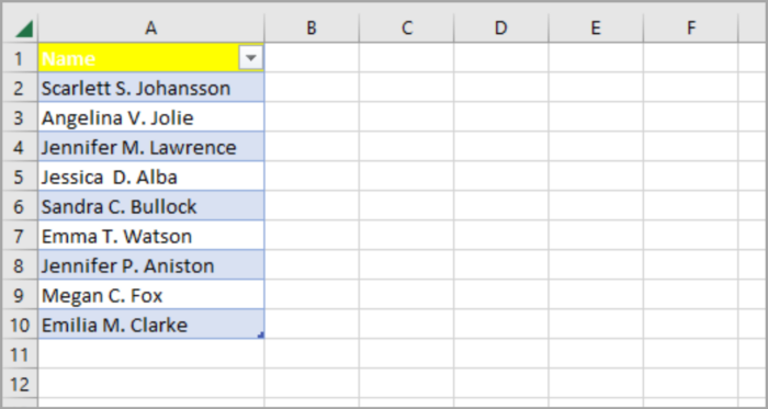
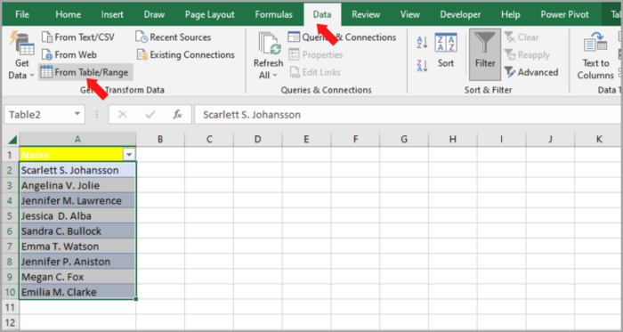
- In your Excel table, select any cell containing your data.
- Go to the Data tab, and click on the ‘From Table/Range’ (under Transform Data group).

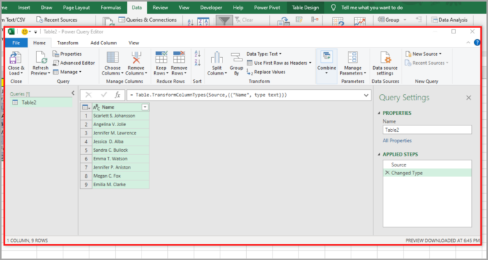
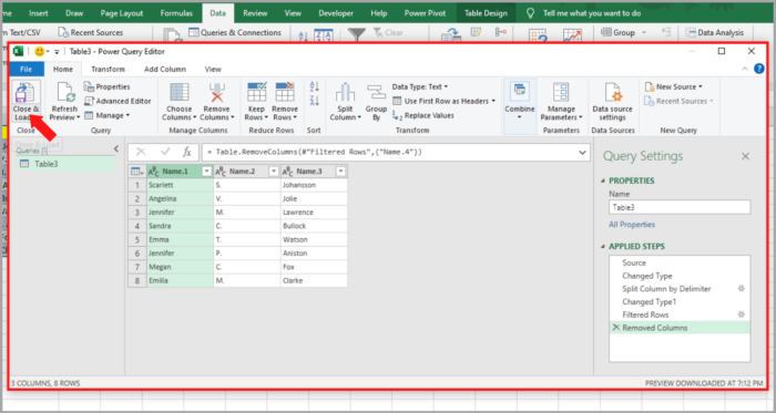
- The Power Query Editor will be opened.

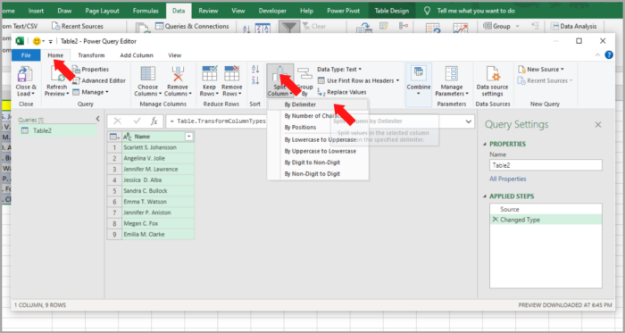
- In your Full Name column, click any cell and click the Split Column drop-down (under the Home tab).
- The drop-down menu appears, select ‘By Delimiter’.

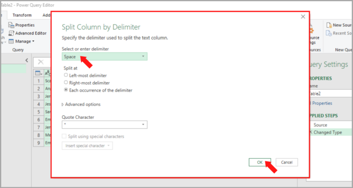
- The dialog box of Split by Column Delimeter will open.

- Keep the Space option selected (under Select or enter delimiter) since your delimiter is a Space.
- Keep the ‘Each occurrence of the delimiter’ radio button selected (under ‘Split at’).
- Then, click the OK button.
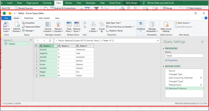
- Now this will separate the Full Name column into three parts.
- Click on the column headers and change them to the appropriate header names as shown in the image below:

- Under the Home tab, click on the Close & Load button.

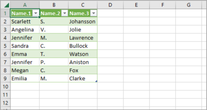
- This will create a new sheet in your workbook containing separated name columns.

Method 5: Use Formula to Separate Names in Excel
This method uses a formula for splitting names in Excel.
This is probably the most challenging method of splitting names. Some parts of the names are extracted and can be used in further processes. This might be handy if you know the formulas in Excel.
Let’s discuss how to extract the first, middle, and last names:
First Name Extract Formula
Here is the formula to extract the first name:
| =LEFT(name_string, SEARCH(“”, name_string) – 1 |
The name_string should be replaced with a reference to the cell containing the name as shown in the above formula.
Simply type the formula below in cell B2:
| =LEFT(A2, SEARCH(“”,A2)-1) |
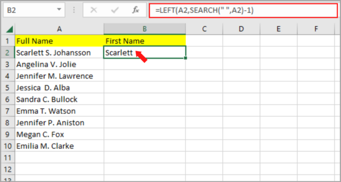
Now, copy the formula to the rest of the cell by double-clicking the fill handle or dragging it down. Here’s the result:
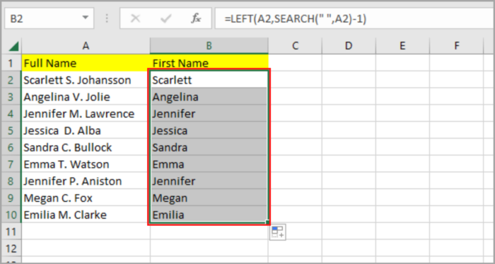
Last Name Extract Formula
Here is the formula for the last name:
| =RIGHT(name_string,LEN(name_string)-SEARCH(“@”,SUBSTITUTE(name_string,” “,”@”,LEN(name_string)-LEN(SUBSTITUTE(name_string,” “,””))))) |
If you want to appear the last name into column D, use this formula in D2:
| =RIGHT(A2,LEN(A2)-SEARCH(“@”,SUBSTITUTE(A2,” “,”@”,LEN(A2)-LEN(SUBSTITUTE(A2,” “,””))))) |
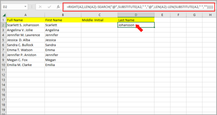
Press enter and copy it to the rest of the cell using the Fill handle by double-clicking or dragging it down. Here’s the result:
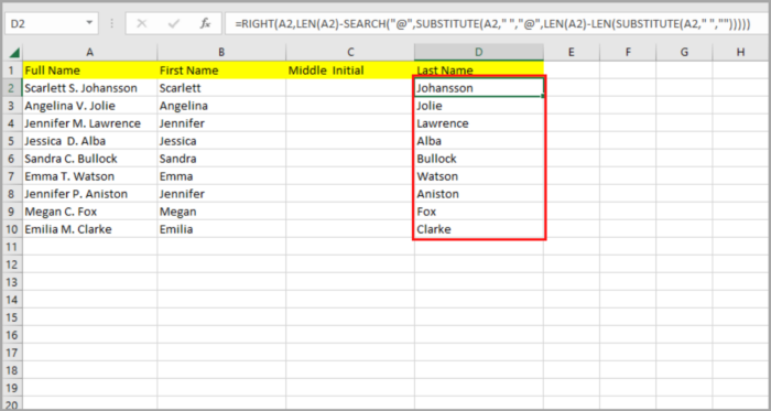
Middle Name Extract Formula
The following is the formula to be used in taking out the middle initial from a given name thread:
| =MID(name_string,SEARCH(” “, name_string)+1,SEARCH(” “,SUBSTITUTE(name_string,” “,”@”,1))-SEARCH(” “, name_string)) |
In our illustration, you can tabulate the formula below in cell C2 to display the middle initials in column C:
| =MID(A2,SEARCH(” “,A2)+1,SEARCH(” “,SUBSTITUTE(A2,” “,”@”,1))-SEARCH(” “,A2)) |
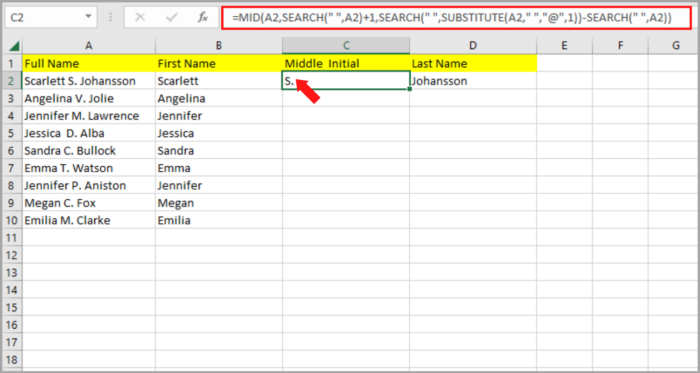
Hit the Enter Key. Drag down the flash-fill function to apply the formula to the preceding cells.
This should be the result:
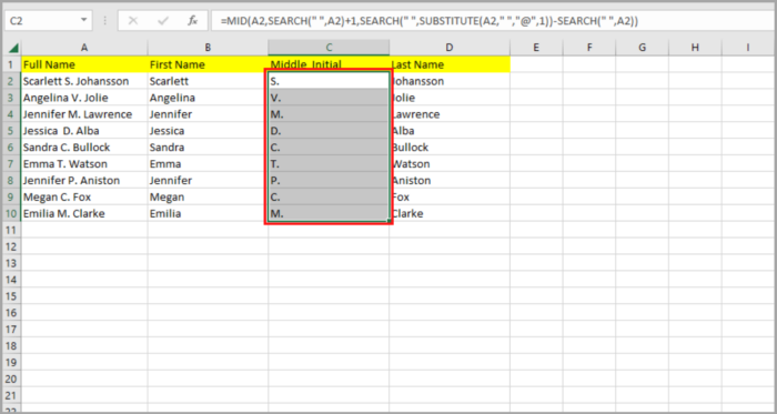
In this article, we illustrated the 5 methods how to extract names in Microsoft Excel, together with the different cases that show the first name, middle initial or middle name, and last name.
Hoping that this tutorial is helpful to you.

