Guide to Removing a Text Prior to or After a Special Excel Character4 Methods with Screenshots & More!


There are certain scenarios you will face when you have to work with data in Excel where you encounter both texts and special characters.
Some cases require you to extract the text before a special character in a text string, or after that.
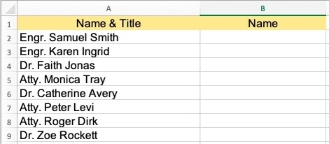
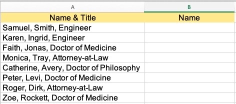
Suppose you have titles of persons prior to their names and you want only to keep their names.
Removing the titles manually is time-consuming.
Removing the text can be accomplished using a formula or the Find & Replace function.
This tutorial will discuss four ways to do this:
- Using Find & Replace
- Using a Formula
- Using Flash Fill
- Using VBA
Using Find & Replace
The Find & Replace function is a simple process that will allow Excel users to either retain the text before a special character or after a special character.
Take the example below:
Simply follow the steps below:
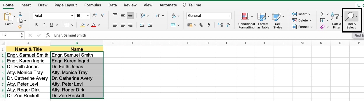
- Copy the values in Column A and paste them into Column B.


- Select the values copied to Column B. Click on Home, locate, and click Find and Select in the Editing group.

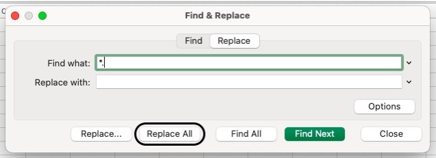
- In the option that appears, click on “Replace”. This will take you to the dialog box Find & Replace.


- Enter “*.” in the field “Find What” and keep the Replace with field empty. Proceed to click on Replace All.

Typing the asterisk before the special character “.” and leaving the replace with field blank removes the period and all of the text prior to it. See below for the output:

In case you wish to remove the characters after the period, you may enter “.*”.
The asterisk here is considered a wildcard character and represents any character.
Using it replaces all the characters after it.
Using a Formula
If you are more comfortable using a formula instead of the Find & Replace function, you may opt to do so.
Let us consider the below example:

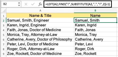
Follow this formula to remove the titles after the names:
![]()
![]()
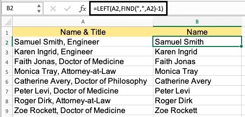
How this formula works is that LEFT refers to the text values that need to be removed before the comma, while FIND locates where the comma is located within the cell.
The -1 entered means that all the values to the left of the comma need to be removed.
The above example is relatively easy.
Let’s say we have the below example instead:
Assuming after the second comma, you wish to extract all the values, the formula to execute this will then be:
![]()
![]()
Having multiple commas means there that the text character to the left of it will be impossible to find and extract by simply using the Find Function.
What I am trying to do here is to extract the data to the second comma’s left.
The exclamation point, which is a special character, will do this for me. It will now be able to extract the data to the second comma’s left.
Another problem that could come up is if the data in the cell has comma inconsistencies.
Let’s say there are two commas in some cells while other cells contain three.
See the example below:
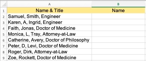
The solution for this is to determine the position of the comma’s last occurrence and to remove the rest of the characters to its left using the formula below:

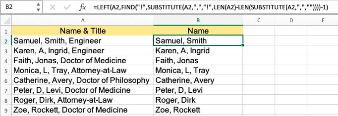
The formula above is the same as the example above but with the Function “LEN”.
This function is used to determine the text’s length within the cell and the text’s length minus the comma.
The total commas in a cell are determined when both the values mentioned above are subtracted.
Use of Flash Fill
This Excel feature is available in Microsoft Excel 2013 up to later versions.
This works by Excel recognizing patterns and then applying them.
First, you have to enter the data a couple of times manually for the pattern to exist.
Take the example below:
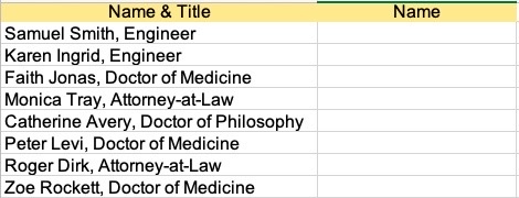
After the comma, if I want to extract the text, here are the steps that I should do with the use of the Flash Fill:
- Enter the name of Samuel Smith and Karen Ingrid in cells B2 and B3, respectively.


- Select B2:B9.


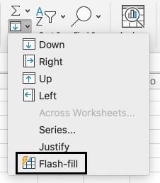
- In Home, click on Fill to see the drop-down results.


- In the drop-down list, tap on Flash Fill.

After clicking on flash-fill, you will now have the below results below:

Another way to use flash fill is to use a keyboard shortcut Ctrl + E.
While it is convenient to use Flash Fill, the results will not always be correct so you still have to do a manual checking if the results in the cells are correct.
Using VBA
This is a custom function and largely depends on Excel’s ability to determine where the comma’s position is.
If you find this, you will be able to string formulas to get you what you need.
But instead of writing long formulas, this process can be simplified using VBA.
Refer to the below code to do this:
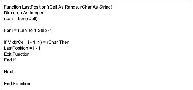
This code should be added to VB Editor’s regular module or in a Personal Macro Workbook.
When you’ve added it, it can be used as any other function in an Excel workbook.
There are two arguments that are followed here:
- Cell Reference (to determine a text string or character’s occurrence)
- Text String (what you want to find)
Once the above code is added to your Personal Macro Workbook, you can type this formula:
![]()
![]()
This formula is simpler and saves you a lot of time instead of those lengthy formulas we have highlighted earlier.
Adding the above code in the Personal Macro Workbook will allow you to utilize this function in all of the Excel workbooks instead of only just one.