Remove Table Formatting in ExcelStep by Step Instructions with Screenshots


Working on a lot of data and information has been made easier through the help of Excel.
What has made it an even more important data source is the use of Power Pivot and Power Query by obtaining information from Excel tables.
What this article will cover is providing a guide to help people deal with removing table formatting and applying customizations, which is a source of frustration for many.
What usually happens is that upon conversion of a data range into an Excel table, there is already formatting applied.
The same happens when an Excel table is formatted back into a table range.
Removing Excel Table Formatting (And Keeping the Table)
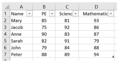
Take the below table as an example:

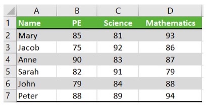
When this data is converted into an Excel Table (shortcut: Control+T), a table like the one below will be shown as:

The table above shows that Excel has automatically applied formatting to the table.
Some people do not like the formatting and might want to change it or apply other customizations.
The next sections will show you how to remove the formatting or change the way the table looks.
Removing Excel Table Formatting
The steps to be followed when removing excel table formatting are as follows:
- In the Excel table, select any cell.
- Click on the Design Tab.


- Under the Table Styles, click on the More button.
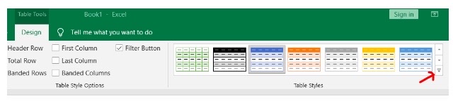

- At the bottom of the Table Styles, click on Clear.

Applying the steps above will remove the automatic formatting of Excel but still keep it as a table.
As shown below, the filters remain and only the formatting has been removed:
Changing Formatting in Excel Table
Manual formatting is an option or you can choose from the presets under Table Styles.
Here are the steps to do it:
- Click on any cell in the Excel Table.
- Click on the Design Tab.
- Under the Table Styles, click on the More button and select a design from any of the presets provided.
- When hovering over a design, you will be able to see what each table will look like.

Removing Excel Table (Converting to Range) & Table Formatting
The conversion from data to an Excel table is as equally easy as converting back the table to a regular table range.
But another point of frustration is when the table formatting is also left out.
The Excel table below can be converted back into a range.

The steps to do that are shown below:
- Select any cell on the table and right-click.
- Choose the Table option and click on Convert to Range.
Notice how the formatting stays after converting the table back into a range as shown below:
To remove the formatting, the following steps can be followed:
- Select the entire range that has formatting.
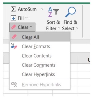
- Click on the Home tab.
- In the Editing options, click on Clear.
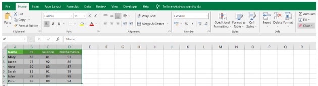

- Click on Clear Formats. This removes any formatting that the range has.
Table Deletion
This probably is the easiest way to do it.
To delete a table, follow these steps:
- Select the data that you want to get deleted.
- Click on Delete. This removes the table as well as all of the formattings on the table.
In case the formatting was applied manually and you wish to remove it from the table, the following steps are to be followed:
- Select the excel table.
- Click on the Home Tab. From there, click on Clear, and then Clear All.