Three Easy Ways to Find Outliers in Microsoft ExcelTutorial with Screenshots


When it comes to data analysis, the assumption is that the data values are close to the mean or median.
However, it can occasionally deviate greatly from the mean or median.
The values are then known as outliers and can give false conclusions from your analysis.
How to Find Outliers Using the Interquartile Range in Microsoft Excel
An indicator of the beginning and end of the majority of your data is the Interquartile Range (IQR).
An outlier is any value that is outside of this range.
The first and third quartile of the data is very important in calculating the IQR. The formula of IQR is
| IQR = Q3 – Q1 |
Where
- Data’s first quartile is designated as Q1.
- The Third quartile of the data is denoted as Q3.
A quartile comprises a quarter of the data value. It is organized from the smallest to largest values of the data.
The first quartile (Q1) comprises the 25% lowest data.
The third quartile (Q3) comprises 50% – 75% of the data and it is classified above the median.
The QUARTILE.INC function in Excel easily calculates the quartile values. The formula used is :
| QUARTILE.INC(array, quart) |
Where
- array – this contains your data (range of cells)
- quart – a value indicating the desired quartile to be calculated
You must set the quartile parameter to 1 in order to calculate the first quartile. Similarly, you must set the quartile parameter to 3 in order to calculate the third quartile.
The smallest and highest values of the permitted data range can be determined using the Q1, Q3, and IQR values, which you can obtain after you have the Q1, Q3, and IQR values (also known as the Lower bound and Upper bound respectively).
Therefore, outliers are any value that is either smaller than or larger than the lower or upper bound.
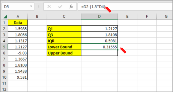
Multiply the IQR value by 1.5 and then deduct it from the Q1 value so that we can determine the lower bound limit:
| Lower Bound = Q1-(1.5 * IQR) |
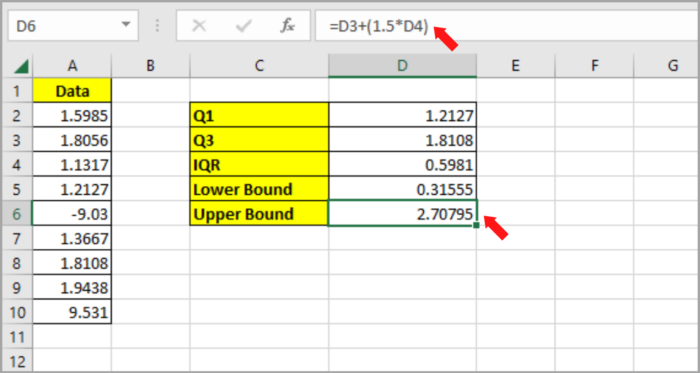
Similarly, we can determine the upper bound limit by adding the Q3 value to the IQR value after multiplying it by 1.5:
| Upper Bound = Q3+(1.5 * IQR) |
Here is the computation sequence to find outliers of your data:
- Use the QUARTILE function in computing Q1 and Q3.
- Subtract Q1 from Q3 to compute the IQR.
- Multiply the IQR by 1.5 and subtract it from Q1 to compute the Lower bound.
- Multiply the IQR by 1.5 and add it from Q3 to compute the Upper bound.
- To find the outliers, locate the points that are greater or less than the lower or upper bound.
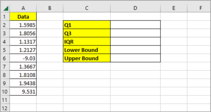
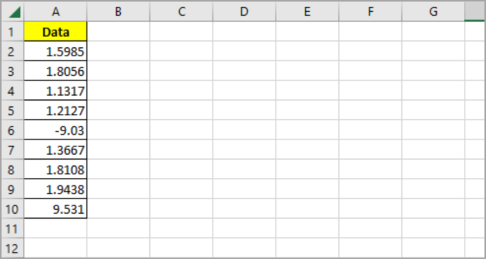
Here is the given data that we will use for the illustration of this problem:

Here are the steps in finding the outliers in the given list:
- First, you need to create a table beside your data list as the one we can see below:

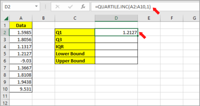
- Type the formula in cell E2 to compute for Q1 value: =QUARTILE.INC(A2:A10,1).
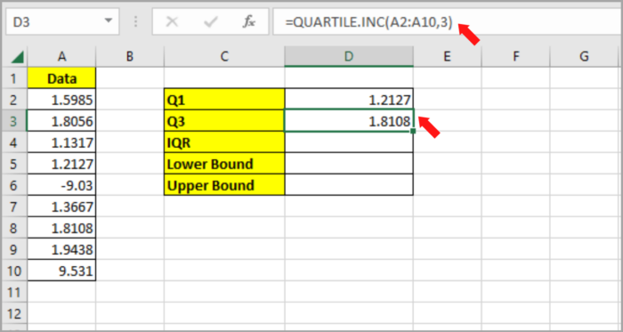
- Type the formula in cell E3 to compute for Q3 value: =QUARTILE.INC(A2:A10,3).
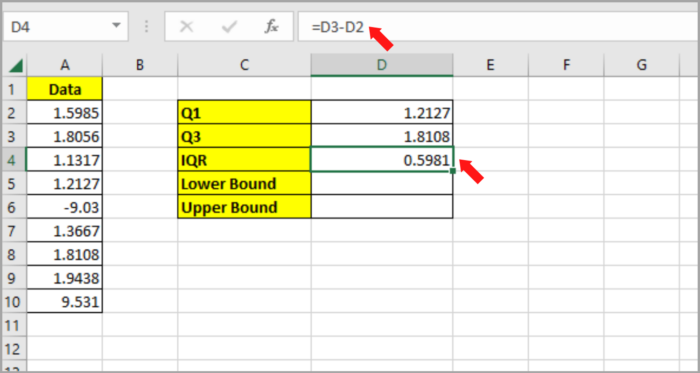
- Type the formula in cell E4 to compute for IQR value: =D3 – D2.
- Type the formula in cell E5 to compute the lower bound value: =D2-(1.5*E4).
- Type the formula in cell E6 to compute the upper bound value: =D3+(1.5*D4).
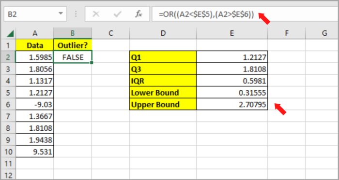
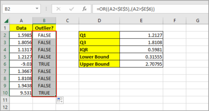
- To confirm if the data is an outlier in the given data, type the formula in cell B2: =OR((A2<$E$5),(A2>$E$6)). If the value is an outlier, it will return TRUE. If not, it will return FALSE.
- By dragging down the fill handle in B2, you can copy the formula to the rest of the cells in column B.
Use the Mean and Standard Deviation in Microsoft Excel to Find the Outliers
The Standard deviation of the data distribution is another simple way of finding outliers.
A standard deviation is a number that describes how widely apart the points in a distribution are from the distribution’s mean value.
If it is 2 to 3 times the standard deviation, we usually assume it to be an outlier.
To compute the Standard deviation of data, the STDEV.S function is used in Excel.
The formula for the function is:
| =STDEV.S(number1,[number2],…) |
The number 1, number 2, etc. are references to each cell in a range.
The mean of the distribution is also needed. By using the AVERAGE function, you can compute the mean. Here’s the formula:
| =AVERAGE(number1,[number2],…) |
The number 1, number 2, etc. are references to each cell in a range.
The outliers are the values that are 2 standard deviations away from the mean. The mean is 2 times less than the mean or 2 times greater than the mean.
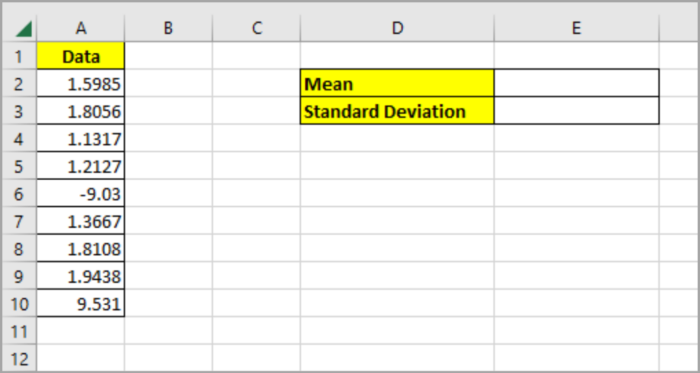
Here is a sample data sheet for this problem:
To find the outliers, we will be using the Mean and Standard Deviation of the data above:
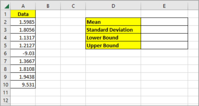
- First, you need to create a table beside your data list as shown below:
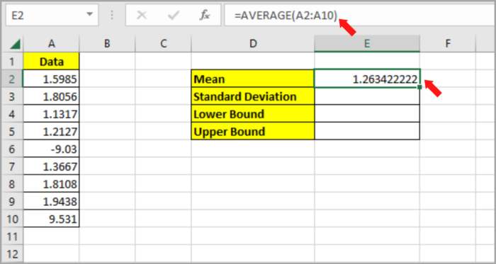
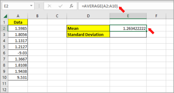
- Type the formula in cell E2 to compute the Mean: =AVERAGE(A2:A10).
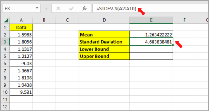
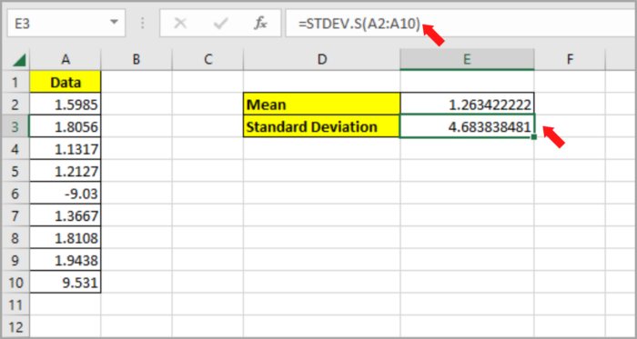
- Type the formula in cell E3 to compute the Standard Deviation: =STDEV.S(A2:A10).
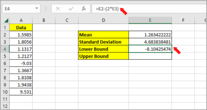
- Type the formula in cell E4 to compute the lower bound: =E2-(2*E3).
- Type the formula in cell E5 to compute the upper bound: =E2+(2*E3).

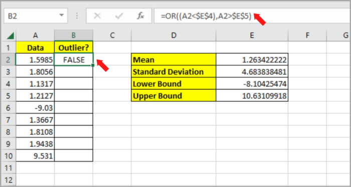
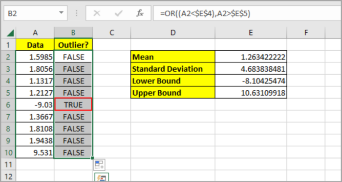
- To confirm if the data is an outlier in the given data, type the formula in cell B2: =OR((A2<$E$5),(A2>$E$6)). If it is an outlier, the result will return TRUE. If not, it will return FALSE.
- By dragging down the fill handle in B2, you can copy the formula to the rest of the cells in column B.
How to Find Outliers Using the Z-Score in Microsoft Excel?
Using the Z-score value is another way of finding the outlier.
This gives you a hint of how far the data point is from the Mean. It is also known as the Standard Score.
In Computing the Z-score, the Mean and Standard Deviation of the data distribution is needed.
Here is the formula of the Z-score:
| Z = (X – mean) / Standard Deviation |
Here,
- X – The individual data value in the distribution.
Z-scores of +/-3 or more from zero is a common cutoff for identifying outliers. Therefore, any value with a Z-score between -3 and +3 can be categorized as an outlier.
Let us also use the given data set below:
Here is the method on how you can use the Z-score to find the outlier in the given data:
- First, you need to create a table beside your data list as shown below:
- Type the formula in cell E2 to compute the Mean: =AVERAGE(A2:A10).
- Type the formula in cell E3 to compute the Standard Deviation: =STDEV.S(A2:A10).
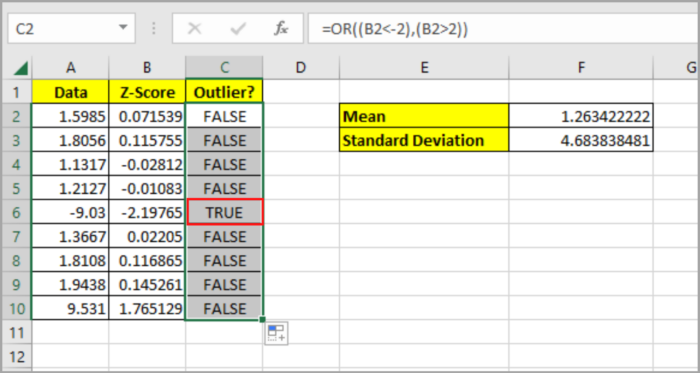
- Calculate the Z-score for each of the data values and then copy it to the rest of the cell in column B. Use this formula in cell B2: =(A2-$F$2)/$F$3.

- As you can see, the Z-score has not crossed the -3 or +3 mark. However, we can tweak the Z-score down to -2 or +2. In this case, we can assume that our outlier is the value that exceeds -2 or +2.
- To confirm if the data is an outlier in the given data, type the formula in cell C2: =OR((A2<$E$5),(A2>$E$6)). If the resulting value is an outlier, it will return TRUE. Otherwise, it will return FALSE.

- By dragging down the fill handle in C2, you can copy the formula to the rest of the cells in column C.
In Excel, there are other ways in finding the outliers of a given data.
We have tackled the 3 easy ways in this tutorial.
Just select what method you prefer in using in your project.