How to Consolidate or Merge Excel Rows While Retaining Data4 Different Ways!
This tutorial will present four secure methods for merging Excel rows, including merging multiple rows while avoiding loss of data, joining duplicate rows, continually merging groups of rows, and copying rows that match from a separate shared columns table.
Combining rows in Microsoft Excel is a frequent requirement, yet the software needs a dependable method to accomplish it. Using the default Merge & Center option can result in an error message as shown in the image below:

Choosing “OK” will combine the cells, however, it will result in only retaining the initial cell’s value, causing all other information to be lost.
Clearly, a more effective solution is required.
This article outlines several techniques that enable merging several rows in Excel while preventing data loss.
Methods for Merging Excel Rows & Prevent Data Loss
The objective: you possess a database with each row maintaining specific details that include product name, customer name, product key, etc.
The goal is to merge all of the rows associated with a specific order as demonstrated:
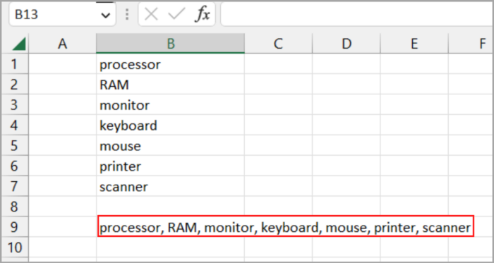
Two methods to accomplish this:
- By using a formula
- Merging cells using an add-in
Using Formulas
Utilize the CONCATENATE function or concatenation operator (&) to combine the values from multiple cells into one.
The CONCAT function is also available in Excel 2016 and beyond. In both cases, cell references are provided and separators are added as desired.
Combine rows and use commas and spaces to separate the data:
| =CONCATENATE(A1,”, “,A2,”, “,A3) |
| =A1&”, “&A2&”, “&A3 |
Combining the rows and using commas rather than spaces to separate the data:
| Combine rows with spacing between the data. |
| =A1&” “&A2&” “&A3 |
Merge rows and separate the values with commas without any spaces:
| =CONCATENATE(A1,A2,A3) |
| =A1&”,”&A2&”,”&A3 |
In real-world scenarios, concatenating more cells is often necessary, making the formula lengthier.
| =CONCATENATE(A1,”, “,A2,”, “,A3,”, “,A4,”, “,A5,”, “,A6,”, “,A7,”, “,A8) |

Having merged multiple rows into a single row, the combined rows now contain formulas. To transform them into values, utilize the Paste Special function.
Merging Cell Using Add-in
Excel’s Merge Cells add-in is a versatile tool for merging cells that may combine both individual cells and whole rows or columns.
Notably, it preserves all data even when the selection has multiple values.
Here is the step-by-step process for merging multiple cells:
- Choose the cell range where the merging of rows is desired.
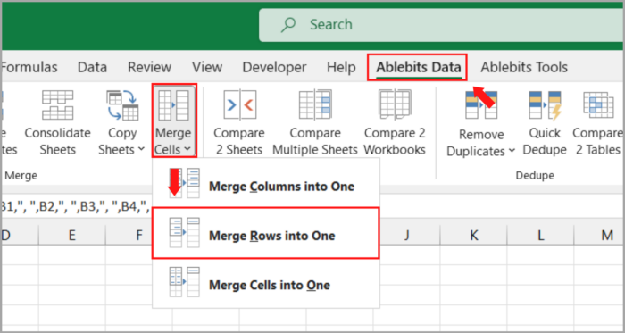
- Navigate to Ablebits Data tab -> Merge Cells -> select “Merge Rows into One.”

- By doing so, the dialog box for Merge Cells will open with the default settings, which are suitable for most situations. As demonstrated in the picture below, we merely switch the separator in this case from the standard space to a line break.

- When you click the Merge button, you’ll see completely combined data rows with line breaks:

Creating a Single Row from Multiple Duplicate Rows While Preserving Only Unique Values
Your goal: you have an Excel database with a few thousand records. While the information in other columns differs, the values in one column are virtually the same.
Your objective is to create a comma-separated list by combining data from duplicate rows depending on a specific column.
It may also be desirable to merge only unique values, excluding duplicates and ignoring empty cells.
Here is the image:

You definitely want to steer clear of the idea of manually locating and combining duplicate rows.
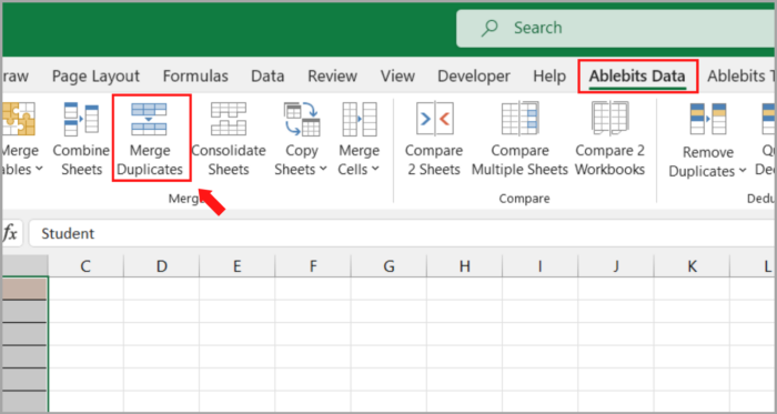
Discover the Merge Duplicates add-in, which streamlines this laborious and time-consuming task into a straightforward 4-step procedure.
- By choosing the duplicate rows you wish to combine, you may launch the Merge Duplicates wizard by selecting its ribbon button.

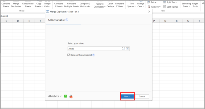
- Click Next after ensuring your table is properly selected. Keep the “Create a backup copy” checkbox selected, especially if this is your first time using the add-in.

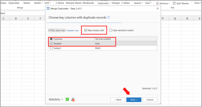
- Select the column used to identify duplicates. Using this scenario, we will choose the column “Customer” as we aim to merge rows based on customer names. Should you prefer to skip blank cells, click on this option and proceed to the next step.

- Pick the columns containing data that need to be combined and specify a delimiter, such as a comma, semicolon, line break, space, etc.
There are two more choices in the top section of the dialog that allow you to do the following:
- Eliminate duplicate values during the merging of rows
- Ignore blank cells
Once complete, click on Finish.

In a short amount of time, all the information from repeated rows will be combined into a single row.
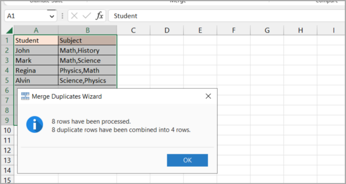
Repeatedly Combine Row Groups into a Single Row
The objective: Combine every set of three rows in a file in Excel into a single row, containing information such as the product & customer names, and purchase date for each order.
Here is an example:
- Create a helper column in your worksheet, in this case, column C. Let’s call it BlockID or anything you want to call it.
- In Cell C2, insert the formula shown below and then drag the fill handle to duplicate it along the column:
| =INT((ROW(C2)-2)/3) |
Where:
- The formula is entered in the first cell of the helper column, which is C2.
- The data begins on row 2.
- Each block consists of 3 rows that are going to be combined.
This formula assigns a unique identifier to each group of rows, demonstrated in the illustration below:
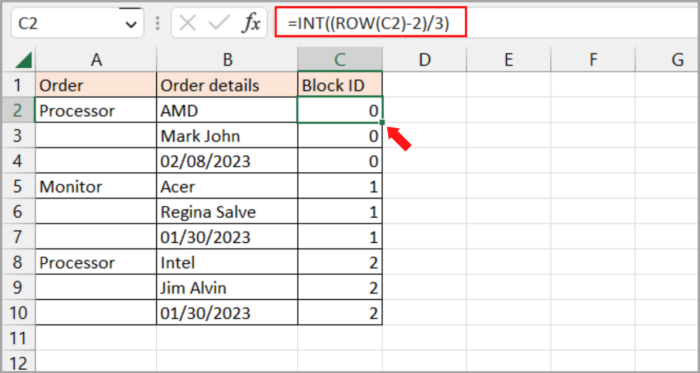
How it works: The formula starts counting from zero by extracting the row number of the formula cell from which you deduct the position of the row where the start of your data is. For instance, since our data begin in the second row, we deduct 2. Your data will have ROW(C5)-5 if it begins, let’s say, in row 5. Then, using the INT function to round the result to the closest integer, divide the aforementioned equation by the number of rows to be combined.
3. Well, the majority of the work is done and you are now ready to bring all the data together according to the BlockID column. To achieve this, use the Merge Duplicates add-in that we’ve utilized previously for merging rows that have duplicates.
- In the second step, select the key column as BlockID.
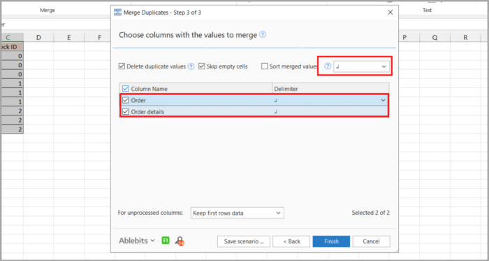
- In the third step, choose the columns that you wish to combine and opt for a line break as the separator.
 Here is the result:
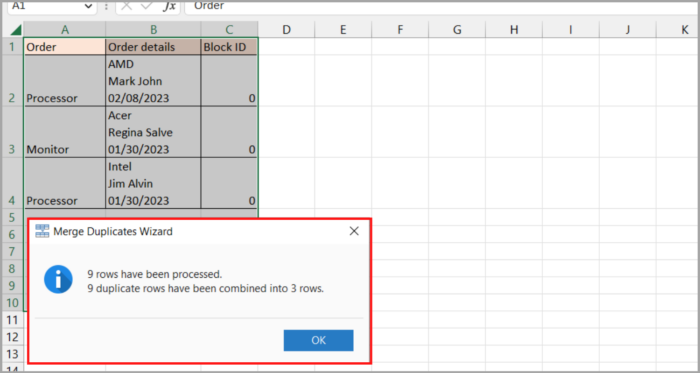
4. The final step is to remove the Block ID column as it is no longer required. And voila! The process of merging blocks of rows into one row is complete, just as in the previous examples, taking only 4 steps.
How to Combine Similar Rows from Two Excel Tables Without the Need to Copy and Paste
The objective: To combine the rows that match in both tables based on a shared column or columns.
The tables may be found on one sheet, two separate spreadsheets, or two separate workbooks.
The goal is to merge the sales reports for the months of January and February, which are located in two separate worksheets.
However, the order of rows and products may differ between the two tables, making simple copying and pasting not feasible.

In this situation, the add-in Merge Two Tables will be a perfect solution, here’s how:
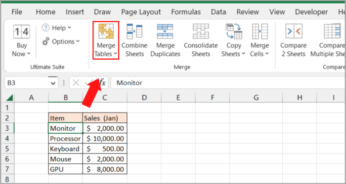
- Click the button Merge Two Tables on the Ablebits Data tab’s Merge group after selecting any cell in your primary table:
 As a result, the add-in will begin with your primary table already chosen, allowing you to go on to the following phase by selecting “Next.”
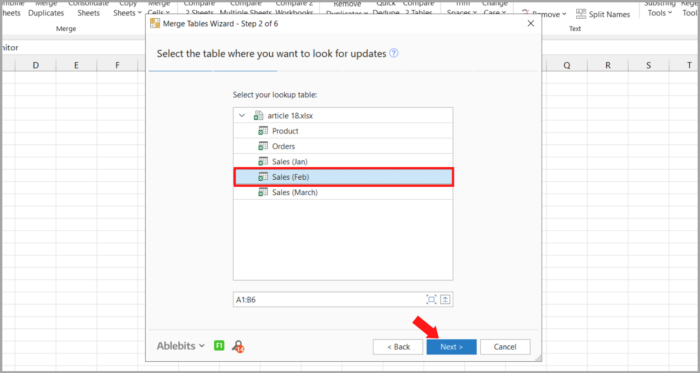
 - Next, choose the lookup table that holds the rows that match.

- Identify columns from both tables to use as key columns, which should have unique values (such as Product ID as an example).

- If desired, in the main table, select the columns to update. If not, proceed to the next step by clicking “Next.”
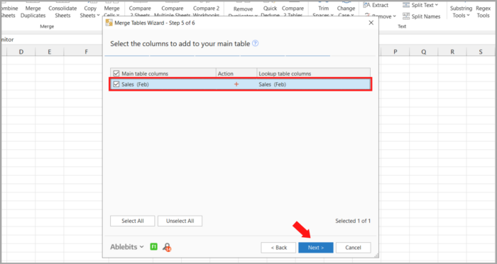
- Choose which columns—in the example, Feb sales—from the lookup table to include in the main table.

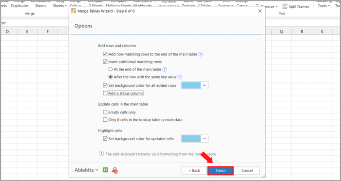
- Finally, select any desired additional options and click “Finish” to complete the merge. The default settings, as shown in the screenshot, will suffice in most cases.

Give the add-in some time to work its magic, then take a look at the outcome:
I hope this tutorial helps you a lot!



 Here is the result: