How to Make an Interactive Calendar in ExcelFormulas, Screenshots, and More


When it comes to preparing for our busy lives, a calendar is a must, and for those of us with a bit of skill at using Microsoft Excel, there is no better tool to prepare for the days ahead.
With only a few steps, you can use Excel to create an interactive calendar that automatically adjusts for changes in months and years.
This is an incredibly useful tool both for accessing your schedule from your devices and for printing your calendars out on paper.
So, without further delay, let’s take a look at how you can create an interactive calendar with Excel.
How To Create an Interactive Monthly Calendar in Excel
There are two common approaches to creating an interactive calendar, and this is to make it a monthly calendar or a yearly calendar.
First, we will take a look at how to create a monthly calendar and then move on to a yearly calendar.
Step 1

The first step is to begin creating two data sets beginning with a list of the months in a year.
In addition to this, if you would like to include a list of federal holidays, follow this by creating a list of all the federal holidays for 2023 as well.
Step 2
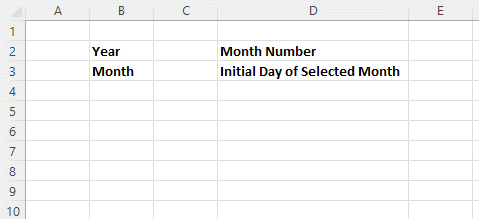
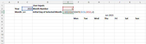
Create fields for the user inputs needed to make the calendar interactive.
This includes Year, Month, Month Number, and First Day of the Selected Month.
Step 3
Now enter the year you will be using for the calendar into the appropriate field, and then select the cell for the month entry, which in our case is D5.
Navigate to the “Data” tab, and under the “Data Tools” group, click on “Data Validation.”
Step 4

In the “Allow” list choose “List,” and then in the “Source” box, choose the cell range for the list of months you created in the datasheet.
Once you are finished, select “OK.” Now the cell for Month should have a dropdown list with all of the months in the year.
Step 5
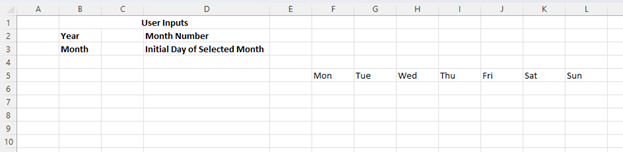
Now you can create the layout for your calendar by creating a 7×7 table in your worksheet.
Place the names for each of the days of the week at the top of the calendar, beginning with Monday.
Step 6
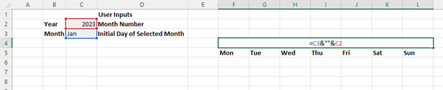
Now to make the header for your calendar dynamic and to do so you will join the cell values for your year and month inputs with the syntax:
=Cell Reference1&” ”&Cell Reference2
This will change the header to match the values of these cells.
Step 7
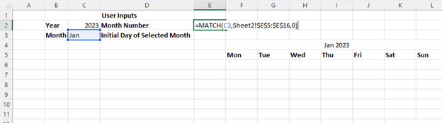
Now inside your designated cell for Month Number, you will need to use the MATCH function to return the position of the month inside your range.
In our case, we will use the formula:
=MATCH(C5,’Sheet2!$E$5:$E$16,0)
By running this formula, it will provide the position of that cell within the data set you created earlier.
This will provide the specific month number, such as in our month 1.
Step 8
Now you will need to make it so that the calendar can determine the first day of each month in a given year and represent each day.
We will use a number from 1 to 7 for each day of the week.
In order to do this, you can use the DATE and WEEKDAY functions.
For our example, we will use the following formula, and you can substitute your particular cell references into the formula.
=WEEKDAY(DATE($C$2,$E$2,1),2)
This will return the number for the specific day of the week, which is, in this case, seven which would equate to Sunday.
Step 9

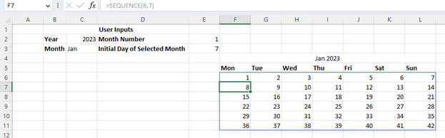
Now it is time to fill in your calendar with numbers, and to do this; you will use the SEQUENCE function on the first cell of your table.
Because your calendar will have six columns as well as seven rows, you can use the formula:
=SEQUENCE(6,7)
This will fill in all of the cells from 1-42 sequentially.
Step 10

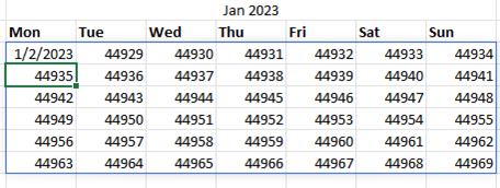
Now you can replace those numbers with a date by using the DATE function.
This can be done by modifying the formula in the first cell of your table to include the DATE function and the information provided by your Year and Month Number cells.
This will be:
=DATE(C2,E2,1)+SEQUENCE(6,7)
Once run, this formula will provide what appears to be a date in the first cell and a series of sequential numbers in each of the remaining cells.
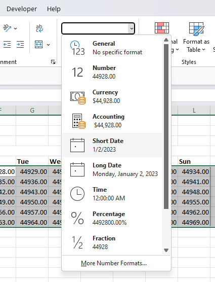
We can solve this by selecting each of the cells in the range and selecting the “Number Format” list and “Short Date.”
You can see now that the dates in each cell are not correctly aligned, but this can be easily solved by updating the formula again.

Now select the starting cell of your table and subtract the value in your Initial Day of the Selected Month field.
Now your formula should read something like this:
=DATE(C2,E2,1)+SEQUENCE(6,7)-E3
Step 11

Now that your dates are correct, you probably notice that you have some days from the previous month listed in your calendar.
Fortunately, you can remove these by altering the formula in your starting cell once again. We will enter the following:
=IF(MONTH(DATE(C2,E2,1)+SEQUENCE(6,7)-E3)=E2,DATE(C2,E2,1)+SEQUENCE(6,7)-E3,””)
After running this formula substituting in your own cell references, you should see all of the extra dates disappear.
Now you should be left with only the appropriate dates in our case, starting with January 1st, 2023, lined up correctly with Sunday.
Step 12
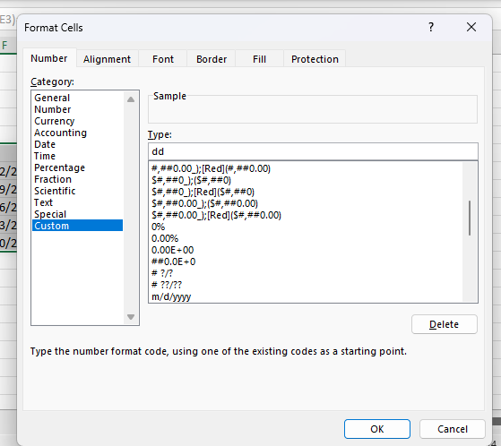
Now it is time to format the dates to look more like a calendar, and to do this, start by selecting all of the cells in your calendar, right-click, and select “Format Cells.”
This will bring up the “Format Cells” window.
Here select “Custom,” and under the “Type” field, enter dd.
Select “OK,” and this will change the format to only display the days.
Now you can also select the cells for the weekends and “Fill Color” under the home tab to give them a different color.
You can do the same with your headers to make them stand out as well.
Now your calendar is interactive and should look pretty good, but you can feel free to resize the cells and change the colors to suit your tastes.
Highlighting Holidays on Your Monthly Calendar
If you would like to highlight all of the holidays on your calendar in a different color, you can do this now.
In order to make this happen, you will need a list of all the holidays you want to be highlighted, which you may have created in step 1 of creating your calendar.
If you did not create this list earlier, then you can still go back and create one now.
Once completed, simply go ahead and follow the steps below.
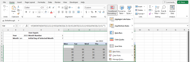
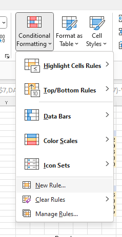
- Select all of the cells in your calendar and select “Conditional Formatting” from the “Styles” group of the “Home” tab. From the dropdown list, select “New Rule.”
- The “New Formatting Rule” dialog box will open, and within the “Select A Rule Type” list, choose “Use a formula to determine which cells to format.”
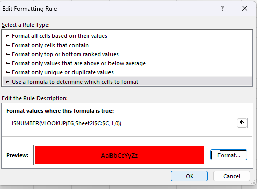
- In the formula box enter the following formula: =ISNUMBER(VLOOKUP(B9,’Data Set’!$C:$C,1,0)).
- Next, click the “Format” button and select the color as well as any other formatting you would like to apply to the holidays. Once you are finished, hit “OK.”
These steps will create a conditional formatting rule that will apply your selected format to the cells based on the dates listed in your data set.
You can test this by checking each month and ensuring any holidays you listed are formatted correctly.
If so, this means that you are finished, and your interactive monthly calendar is complete!
Creating an Interactive Yearly Calendar in Excel
Just like a monthly calendar, it is possible to create an interactive yearly calendar in Excel, and in fact, the steps are very similar.
There are some differences in formatting and creating this style of calendar, however, so let’s take a closer look at the whole procedure.
Step 1

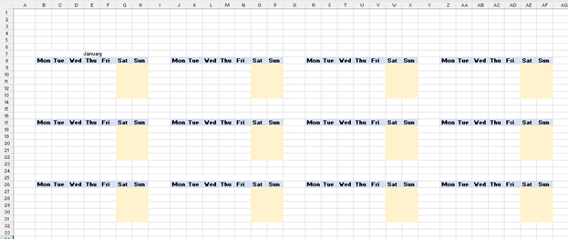
First of all, you will need to create twelve seven by seven tables for each of the months in the year.
In the top row of each of these tables, enter the days of the week beginning from Monday.
In addition, add the year, in this case, 2023, above the cells.
Step 2
Now in a cell positioned above your first seven-by-seven table, type the numeral 1.
Feel free to center this above your table using “Center Across Selection” and then right-click on the cell.
From the context menu, select “Format Cells.”
Step 3
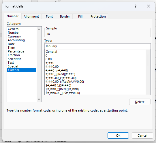
This will open the “Format Cells” dialog box where you will navigate to the “Number” tab; select “Custom” from the category list, and under the “Type:” selection, enter January.
When you are finished, select “OK.”
You should now see January as the header for the first table.
Step 4
Now you can repeat the same process for each of the remaining tables using the numbers one through twelve and displaying them as the appropriate month.
Feel free to color the background of the headers as well to improve the appearance.
Step 5
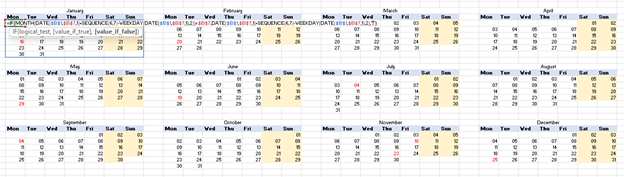
Now it is time to enter the dates into the table for January and to do this, we will use the following formula:
=IF(MONTH(DATE($B$1,$B$7,1)+SEQUENCE(6,7)-WEEKDAY(DATE($B$1,$B$7,1),2))=$B$7,DATE($B$1,$B$7,1)+SEQUENCE(6,7)-WEEKDAY(DATE($B$1,$B$7,1),2),””
Notably, unlike the monthly calendar, we do not have any separate fields for months or years in this sheet.
Instead, all of these formulas are incorporated into this one. Also, this formula uses the top leftmost cell reference, where you entered one earlier, to determine which month we are referring to in lieu of a separate input, which means you may need to substitute a separate cell reference.
Step 6
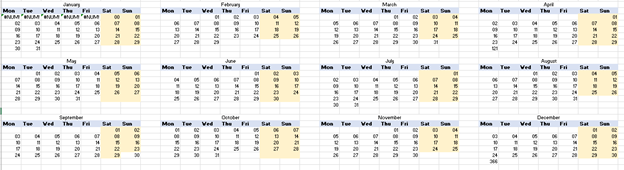
Using the same formula as for January but substituting in the appropriate cell references for each month, enter the days for each remaining month.
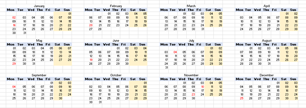
When you are finished, your calendar should look nearly complete, with the exception of the holidays.
Highlighting Holidays on Your Yearly Calendar
There is one last step to accomplish in completing your calendar, and this is highlighting the holidays.
This is performed in essentially the same way as for the monthly calendar.
Similarly, you will need to create a list of the holidays and their dates as described in Step 1 of the monthly calendar for this to work.
Here are the steps to highlight these dates on your calendar.
- Select the cells in your calendar for January and select “Conditional Formatting” from the “Styles” group of the “Home” tab.
- Select “New Rule” to bring up the “New Formatting Rule” dialog box. Then select “Use a formula to determine which cells to format.”
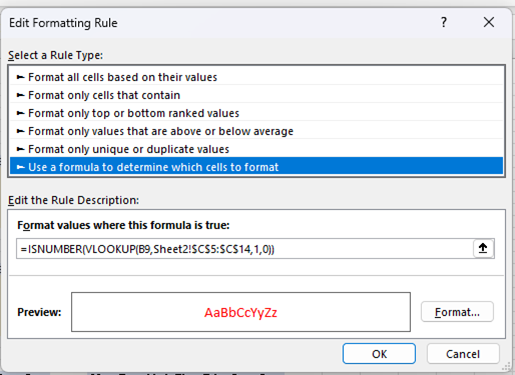
- In the field “Format values where this formula is true,” enter =ISNUMBER(VLOOKUP(B9,Sheet2!$C$5:$C$14,1,0)). Click on “Format” and choose how you would like to format the holidays. When you are done, click “OK.”
- Now repeat the same process with each of the remaining months. However, substitute the top-left cell reference of each month in the formula.

That is it! Now your calendar is complete, and you can change the formatting in any way you like to make it your own.
Conclusion
A calendar is a crucial tool for scheduling our busy lives, and Excel provides the perfect tool for creating a unique calendar that automatically updates to changes in month and year.
By following the steps above, you can easily create a calendar to help you plan ahead.