How To Use INDEX and MATCHDefined with Examples, Step by Step Screenshots & More


When it comes to searching for a particular value in a cell located somewhere in a table, there is a good chance that your first choice would be to use VLOOKUP, and this is certainly understandable.
After all, VLOOKUP is designed to do just this, and it can certainly get the job done, but in many cases, there is a better way.
Excel provides several functions designed to help you find the data you need, and in addition to VLOOKUP, two of these functions include the INDEX and MATCH functions.
These functions work on their own in two very different ways to return data, but when combined, they can create an even more powerful tool.
The INDEX function returns values based on a location that you enter into the formula, while, in contrast, the MATCH function returns a location based on a value.
When these functions are combined into one, it can create an incredibly flexible and powerful search tool that can perform lookups, both vertical and horizontal searches, even using multiple criteria.
This often makes INDEX and Match a more powerful search tool than even VLOOKUP, and it can be extremely helpful to understand how to use this tool if you frequently use Excel to store large amounts of data.
Here we will take a closer look at INDEX and MATCH and how they can be used.
The INDEX and MATCH Functions
INDEX and MATCH are a combination of these two independent functions, which, when combined, creates a powerful two-way search tool.
In order to effectively use these search tools, it is important to understand what both of these functions are and how they work.
The INDEX Function
The INDEX function is an extremely flexible function used to retrieve a value from a location within a specified range.
In other words, to return a value contained in a defined location on your spreadsheet.
Due to its extreme utility, it is often used in combination with other functions within Excel formulas.
The syntax for this function is:
INDEX(array, row_number, column_number)
The first two of these arguments are required, which means the array and the row number.
This will allow you to perform a one-dimensional search for the specified value. However, if you would like to search based on both columns and rows, you can include both of these arguments.
There is one clear flaw to using this function that you have probably already thought of, and that is how often you are looking for a value for which you already know the location in your worksheet.
Fortunately, there is an easy and effective solution to this problem, and that is pairing it with the equally powerful MATCH function.
The MATCH Function
The MATCH function allows users to find the position of a specific value within a defined range of cells.
In other words, if you know the value you are looking for, the MATCH function can tell you precisely where it is located.
The syntax for this function is:
=MATCH(lookup_value, lookup_array, [match_type])
The lookup value is the specific value that you want Excel to find the location for in your data, and the lookup array is the range of cells in which it is located.
The MATCH function is not limited to a horizontal or vertical range and is equally capable of returning values from either.
The final argument in this function, the match type, is important as this argument determines whether or not the formula will provide you with an exact or approximate match.
Potential values that can be entered for this argument include:
- 0: If 0 is entered, the MATCH function will only return the location of an exact match;
- 1: If one is entered, a near-match may be returned rounded down to the nearest available value; or
- -1: If -1 is entered, a near-match may be returned rounded up to the nearest available value.
Unlike the first two arguments, however, you do not need to include a match type.
If you choose to leave this argument blank, then Excel will simply default to 1 and look for an approximate match.
In many cases, this may be okay, but if you are looking for an exact match, then do not forget to enter 0 for the match type to force the MATCH function to return only exact matches.
How To Use Index And Match Together
Now you know what the INDEX and MATCH functions are and how they work, it is easy to see how they can work together extremely well.
When used in combination, these two functions can create a powerful and dynamic lookup tool that is easy to use.
Now that we know the syntax for each of these functions, we just need to combine them, and to do this; the MATCH function is simply inserted into the formula for the INDEX function in place of the lookup position.
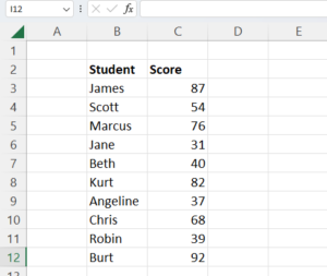
For example, to find the test scores for the student Chris within the worksheet below, we could use a combination of these two functions.
Use the formula:
=INDEX(C3:C12,MATCH(F3,B3:B12))

In this formula, we ask Excel to provide us with the test score for the student Chris using the INDEX function, and we tell it where to find this value using the MATCH function embedded within it in place of the row and column numbers.
Simply by running this formula, we are provided with this student’s test score.

Now instead of using a cell reference to tell Excel what we are looking for, we could instead have included the student’s name directly.
However, when using a specific text value instead of a cell reference, remember to enclose it in quotation marks.
Advantages of INDEX and MATCH Over VLOOKUP
In the example above, INDEX and MATCH were used to easily find and return a student’s test score from a list, but the same task could have easily been performed using VLOOKUP instead.
Though VLOOKUP remains a powerful tool, there are some things that INDEX and MATCH can do that are difficult or impossible to accomplish with VLOOKUP.
For one thing, unlike VLOOKUP, which can only search vertically, INDEX and MATCH is capable of searching both vertically and horizontally.
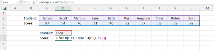
This means that if our student’s test scores were recorded in rows instead of columns, we could still find them using INDEX and MATCH.
We would simply use the same formula but change the range, row, and column parts appropriately to account for the changes in structure as below.
This is already a powerful advantage to using INDEX and MATCH, but it is not the only one.
One of the most powerful other advantages of using a combination of INDEX and MATCH is its ability to perform a left lookup.
This is possible with extreme difficulty and a significant amount of work with VLOOKUP by adapting the formula.
VLOOKUP is only intended to acquire values located to the right. However, in most cases, it is not feasible to do otherwise.
With INDEX and MATCH, though, it is easy to perform a left lookup.
For example, consider if each of the students taking the test came from a different teacher’s classroom.
If our teachers are listed in the column to the left of our students, and we want to find out which teacher belonged to a given student, we could use INDEX and MATCH to find out.
All we would have to do is alter the formula to let Excel know we want to return the value from the column located to the left of our student’s name and run the formula like so.
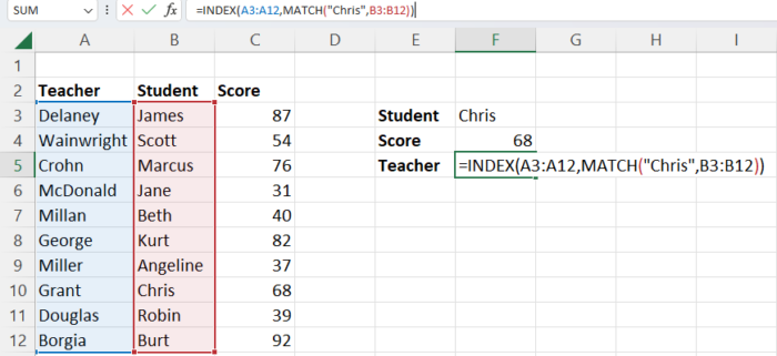
As you can see, it is no more difficult than performing a right lookup, and this gives INDEX and MATCH a considerable degree of flexibility.
Conclusion
Excel provides a number of functions that can help you find the data you need, and perhaps more than any other, the combination of INDEX and MATCH can provide extreme utility and flexibility.
Simply by combining these two distinct functions, it is possible to locate and return data located within both horizontal and vertical ranges anywhere in your worksheet.