IFERROR w/ VLOOKUP to Remove #N/A ErrorsExcel Formula and More


The VLOOKUP formula is one of the strongest tools in many Excel users’ toolkits for finding data in their worksheets.
However, when VLOOKUP is regularly used, it is pretty much inevitable that you will end up with an #N/A error one day.
This occurs because the function is unable to find your specified lookup value.
This can be quite a hassle, but there is no need to panic because Excel provides a handy way to display meaningful results with each occurrence of these errors, and this is the IFERROR function.
When used in combination with VLOOKUP, IFERROR can be used to provide a customized message that looks better and can prove more valuable than a #NA error message.
Here we will learn how to use these two functions in conjunction with each other.
However, first, let’s take a closer look at what the IFERROR function is and how it can be used.
The IFERROR Function
IFERROR is one of a group of error-checking functions that include ISERROR, ISERR, ISNA, and IFERROR. Its purpose is a relatively simple one.
When errors such as #N/A, #VALUE!, and #NULL! occur, the IFERROR function will recognize it and return a message specified by the user.
The syntax of this formula takes the form of the following:
=IFERROR(value, value_if_error)
- Value – This is a required argument that describes the value, formula, or reference that needs to be checked. This is commonly provided in the form of a cell reference. However, when used in conjunction with VLOOKUP, this will be the VLOOKUP formula.
- Value_if_error – This is also a required argument that defines the value that Excel will return if the formula results in an error.
When using this formula, if the specified value is returned as an error, it will return the value specified in the second argument. While using it in conjunction with VLOOKUP, this will occur when the search value is not found in the provided data set, which will result in a #NA error.
An error could occur for several reasons when using the VLOOKUP formula. This includes issues such as:
- Failing to discover the lookup value in the specified array;
- A leading or trailing space in the value or a double space; or
- A spelling error in either the provided lookup value or the array.
No matter the reason for the error, using a combination of the IFERROR and VLOOKUP functions can provide a meaningful result. However, keep in mind that in many cases correcting simple errors such as an additional space or spelling error can still provide a more meaningful result while preventing future errors, particularly when the entry error is in the source data.
Using IFERROR and VLOOKUP to Provide Meaningful Results
Consider a dataset like this one:
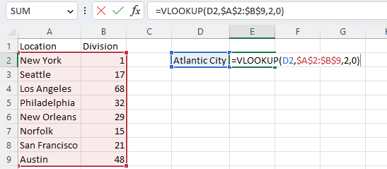
Here we have a list of cities and corresponding division numbers, and we wanted to know what division number belongs to Atlantic City.
However, the VLOOKUP returned a #N/A error because this value was not included in the lookup range.

In this case, it is plain to see that the value is not in the list, but in many cases, data sets could be extremely large, and you may have to check for the occurrence of values regularly. In these cases where a value is not discovered, you will receive a #N/A error.
By enclosing the VLOOKUP formula inside of IFERROR, you can receive a custom response that can provide a much more meaningful or presentable result instead.
The formula to use these two functions together is:
IFERROR(VLOOKUP(…), “Custom Message”)
In our case, we will use the precise formula:
=IFERROR(VLOOKUP(D2,$A$2:$B$9,2,0),”Data Not Present”)
We will simply enter this formula in place of our previous one.
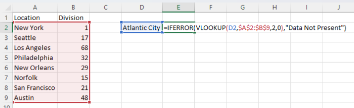
This will return our custom message in place of the N/A/ error.
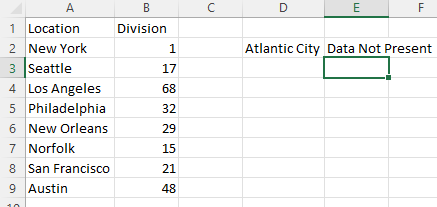
The custom message in our example is “Data Not Present”; however, it can be substituted with any other text you choose.
You could also use zero or simply leave it blank instead of including text or an error message.
As you can see, this is simple to use and can present a much less intimidating-looking result than a N/A error.
This can be far more presentable when presenting an Excel spreadsheet to other users.
However, keep in mind that IFERROR is only available for Excel 2007 and newer.
For older editions, you will need to use the ISERROR function, which works similarly.
Using VLOOKUP With IFERROR To Search Multiple Tables for Results
Consider situations when your data is spread across multiple tables.
What can you do when you perform a lookup of a specific value in one list and cannot find it?
Do you search again and maybe set a custom error message?
The fact is that IFERROR can offer you a way out of this situation that may make your search a little bit easier by nesting an IFERROR formula within another, we can search the first table, and if it returns an error, we can make it so that it will proceed to automatically search the next table.
Let’s assume that using the same example, we have the same locations and division codes, but in addition, we have another list of locations as well. In this case, we can use the following nested formula to search the first list, and if the result is not found, it will search the second list.
=IFERROR(VLOOKUP(D2,$A$2:$B$9,2,0),IFERROR(VLOOKUP(D2,$I$2:$J$5,2,0),”Data Not Present”))

Entering this formula into our worksheet results in a failure to find the result in the location list. So it follows by searching the Additional Locations list.
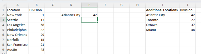
Here it finds the result we were looking for of 42. If it had not found the lookup value, then it would have entered our custom message “Data Not Present.”
When To Use IFNA Instead
IFERROR is a broad tool that will respond to all types of errors, whereas IFNA will only handle #N/A errors.
When you are using VLOOKUP, you will want to consider which types of errors you want to treat.
As we discussed earlier, numerous issues can result in an error, including entry errors for both your formula and the data range, as well as a failure to find the lookup value.
If you do not care about distinguishing between the cause of the error and would like a custom message to be displayed regardless, then use IFERROR.
However, if you would prefer to only treat #N/A specifically, then use IFNA.
This type of error is most likely to result from VLOOKUP failing to find your specified lookup value instead of other types of errors.
Conclusion
As you can see, by using IFERROR in your VLOOKUP formulas, it is possible to provide a more meaningful and presentable response when #N/A errors occur.
This is relatively simple to do and can handle what may otherwise result in multiple searches and a cumbersome troubleshooting process.