How To Lock Formulas in ExcelA Step-by-Step Guide


It is simple to create Excel formulas and edit them as well.
You can edit your formulas by using the formula bar, or you can choose to edit your formula right in the cell.
These options are great for making it easy to create Excel formulas.
But, unfortunately, it’s not so great if you are creating a worksheet with several formulas, then you happen to bump delete, some other keys, or even a combination of keys that could cause problems.
It is possible that you might be able to correct your mistake.
But, then again, you might not be able to fix the problem.
In this case, your worksheet may contain some significant errors. Sometimes these types of errors can even cause businesses to lose money.
These types of mistakes can be even worse if you are sharing your worksheet with your co-workers or maybe even clients.
However, you can stop this from happening.
One thing you can do to stop this sort of thing from occurring is to lock your worksheet along with all of the cells in it.
But, if you do this, Excel will not allow the user to alter your worksheet. This might be a problem if the user needs to make some changes or even add comments.
There are other ways to solve this problem, though, that will work better by allowing you to lock solely the cells with formulas in them.
So, to help you, we will explain how this is done.
Unlock All of the Cells
This step might seem odd since you want to protect your formulas. But, as long as all of the cells are locked, no one will be able to alter anything in the worksheet.
So, in order to change the worksheet so as to protect only the cells with formulas in them, you will need to first unlock all of the cells.
After this, you will be able to take the steps needed to lock the cells with formulas in them.
Here is how to unlock the cells in your worksheet.
- Select all of the cells in your worksheet.
- Once you have selected all of the cells, you can hold down the control key and press the 1 key. You should see the dialog box for formatting cells open.
- In this box, you will want to choose the “Protection” tab.
- Now, find the option for locking the cells and uncheck it.
- Click okay.

Select Only the Cells With Formulas
At this point, the cells should all be unlocked. Now, we want to lock all of the cells containing formulas in them.
To do this, take the following steps.
- Select all of the cells in your worksheet.
- Now, on the “Home” tab, locate the editing group and choose “Find & Select.”
- In the drop-down box, click on “Go to Special.”
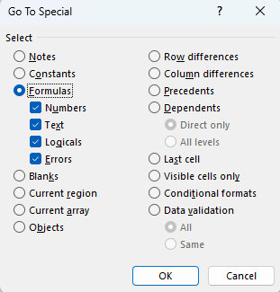
- When the dialog box for “Go to Special” appears, choose “Formulas.”
- Click okay.
By doing this, you have selected only the cells that contain formulas.
Lock the Cells That Have Formulas
In this step, you will lock the cells that have formulas by using the lock feature that you disabled in the first step.
This allows you to protect the cells with formulas without preventing people from altering any other cells in the worksheet. To do this, follow these steps:
- Select the cells containing formulas and hold down Control, and press 1.
- When the format cells dialog box appears, choose the “Protection” tab.
- Choose the option to lock the cells.
- Click okay.

Protect Your Worksheet
Once you are finished protecting the cells with formulas, only the cells containing formulas will be protected if you protect the whole worksheet.
Here is how to protect your worksheet.
- Find the “Review Tab.”
- Click on “Protect Sheet.”
- When the dialog box appears, choose the option “Protect worksheet and contents of the locked cells.”
- If desired, enter a password.
- Click okay.

After you have taken the above steps, all of the cells containing formulas will be locked.
Users will then be unable to change them.
Hide the Cells
Now that you have locked the cells that contain formulas, other people will not be able to alter them.
But, if a cell containing a formula is chosen, the user will be able to see the formula by looking at the formula bar.
If you would prefer the formula not to be seen, it can be hidden.
Follow these steps to hide the cells.
- Select the cells you want to hide.
- Find the “Home” tab and click “Find and Select” in the Editing Group.
- In the drop-down box, choose “Go to Special.”
- When the dialog box appears, choose “formulas.”
- Click okay, and the cells containing formulas will be selected.
- Now, hold down the control key and press 1.
- You will now see the dialog box for formatting cells.
- In this dialog box, locate the “Protection” tab.
- Choose the option “Hidden.”
- Click okay.

Once you complete these steps, if a user selects one of the cells with a formula in it, the formula will not show in the formula bar.
However, remember that you must have a cell locked in order for it to be hidden, just as a cell must be locked in order to be protected.
If you check the box “Hidden” in the “Protection” tab without first locking the cells, it will have no effect.
You must both lock the cells and check the “Hidden” box in order to hide your formulas.
Final Thoughts
There are many times that it can be useful to be able to allow users to make changes to a worksheet without having to worry about having them cause serious errors in your work by accidentally changing your formulas.
By following the procedures above, you should be able to protect your work and still allow others to make needed changes.