How To Insert a Check Mark (Tick Mark ✓) Symbol in ExcelQuick and Easy Guide
A check mark is a commonly required symbol that is useful for giving a professional and clean look to spreadsheets.
As a result, it is commonly required for business professionals and others.
But unfortunately, Excel does not make it as easy to add this symbol as one might expect.
The good news is that there are several ways that you can add a checkmark to your Excel worksheets, and once you do, it is easy to add as many more as you need.
You can also change the appearance of these symbols to match the appearance of the rest of your workbook. Let’s get started.
How Is a Check Mark Different from a Checkbox
In Excel, there are two different types of “checks” that you can add to your worksheet, and it is important to understand the difference to determine which you need.
The process for adding these items is very different, so it is important to make sure of which you need before getting started.
Check Mark
A check mark is a symbol the same as any other text that you would enter into a cell.
A check mark is not interactive and is simply entered into a worksheet as a symbol.
It can be copied with the other symbols present in a cell and pasted into other cells.
In the same way, its font size and other factors of its appearance can be altered and deleted with the other contents in a cell as well.
In this article, we will be looking at how to insert these check marks in Excel.
Check Box
Unlike a check mark, a check box is an object that is not a part of any cell.
A check box sits over a cell and is unaffected by changes to a cell.
For example, when the contents of a cell underneath a check box are deleted, the check box will be unaffected.
This also means that a checkbox can be dragged to move it anywhere on the worksheet without affecting cells.
A check box is interactive and can be selected to add or remove a check mark inside the box.
As a result, it is useful when creating interactive graphs, tables, and reports.
How To Insert a Checkmark in Excel
There are several ways to insert a checkmark into an Excel worksheet.
Here are a few of the most convenient options to use.
How To Insert a Checkmark Using the “Insert” Tab
One of the easiest ways to insert a checkmark manually is to use Excel’s “Insert” tab to add symbols.
Simply follow the steps below to do this.
- Select the appropriate cell. Select the cell where you would like the check mark to appear on your worksheet. To do this, simply click on the appropriate cell to ensure that it is actively selected.
- Navigate to the “Insert” tab. On the top of the ribbon, look for the tab named “Insert.” This will bring you to a menu with a number of different options. Here select the option marked “Symbols” from the ribbon, and from the two options that will appear, select “Symbol” again.

- In the dialog box that appears, select Wingdings under the font options. The font options can be found on the top left of the dialog box, and from here, select Wingdings near the bottom of the list of available fonts.
- Select the check mark symbol to insert. In the list of symbols that will appear, scroll through the options and choose the check mark symbol. This can normally be found near the bottom of the list. Once selected, click “Insert.”
A checkmark will now be added to your active cell.
You can copy and paste this check mark as many times as you need now to get additional marks.
Copy and Paste a Check Mark
Instead of going through the steps above to add a check mark, you could just start by copying one.
A check mark can also be added as simply as finding one from another source and copying and pasting it into your worksheet.
This works because it is regarded as a text symbol.

To do this, start by selecting a check mark such as this one ✓.
Then copy and navigate to the cell where you would like to add it.
Double-click the cell to enter into edit mode and simply paste the check mark.
This method is great for easily adding a check mark when it is only needed a few times.
Of course, since you will need to manually add it each time, and then depending on the source formatting and your own worksheet’s formatting, you may need to adjust the check mark that appears, it may not be the best option if you need to add check marks to a large number of cells.
Insert a Check Mark with Keyboard Shortcuts
One of the quickest ways to add a single check mark in Excel is to use a keyboard shortcut.
To do this, simply follow these steps
- Select the cell where you would like to add a check mark. Make sure that it is the active cell.
- Set your font to “Wingdings 2.” The keyboard shortcut will only work if the font in the cell is set to “Wingdings 2.”
- Hold down “Shift” on your keyboard and press “P.” This will insert a check mark into your cell.
That is all there is to it, and it is a very quick way to add a check mark. The only downside is that you will have to set the font to “Wingdings 2” every time you want to add a check mark.
Insert a Check Mark Using a CHAR Function
Another method to add a checkmark in Excel is to use a CHAR function.
This will create a character in your worksheet based on a specific code you enter into a function.
This clearly may be more complicated at first, but there is a reason you may want to use this method, and that is because it can be integrated into other functions.
This means that, for example, you could tell Excel to input a check mark based on the value in another cell simply by using an “=IF” formula.
The one inconvenience is, however, that you will need to convert the font to “Wingdings” in order for Excel to display a symbol instead of the ANSI character (ü).
So, to use this method, simply enter one of the two formulas below and hit “Enter” on your keyboard:
Use the formula =CHAR(252) or =CHAR(254).
The first =CHAR(252) will return a simple check mark, and the second, =CHAR(254), will return a checked box.
Remember to set the font to “Wingdings” either before or after entering this formula.
Insert a Check Mark Using AutoCorrect
A final and perhaps the quickest way to add check marks is to use Excel’s AutoCorrect feature.
The same program which fixes your spelling mistakes can add check marks to your worksheet for you, and this can be an incredibly fast way to add check marks when you are working.
The only drawback to this method is that it will require a little bit of an upfront time investment.
To do this, you update Excel’s list of expected misspellings that Excel corrects for you to include a word that will automatically be updated into a ✓.
Here is how.
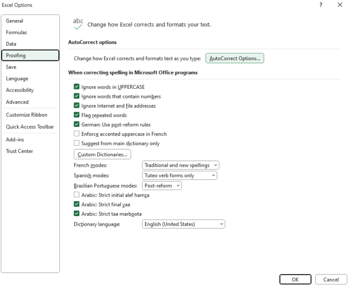
- Open the “File” tab on the top-left of the ribbon and click “Options” on the lower-left-hand side of the menu.

- From here, navigate to the “Proofing” tab and select “AutoCorrect Options.”

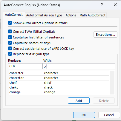
- This will bring up a dialog box, and in the “Replace” box, you want to add a word that will be automatically replaced with a check mark, such as “CHK.”
- Next, in the “With” box, enter a check mark symbol such as this one ✓.
- Select “OK,” and you are done.
Now, whenever you enter the word you have chosen, Excel will replace it with a check mark.
Keep in mind that AutoCorrect is case-sensitive, so it will not convert your chosen word if, for example, you left caps lock on.
However, this method is a great way to make it easy to add check marks as you are working with only a little upfront investment of time.
How To Adjust the Appearance of a Checkmark in Excel
Once added, a check mark functions the same as any other text in Excel.
This means that you can change its appearance freely to fit your needs.
The size and color can be changed to make it more prominent or subtle, and the font can even be changed.
A common way to adjust a check mark once added is to change the color to green to make it more noticeable.
However, you could also adjust the cell background to green and the font color to white for an even more prominent effect.
You may also choose to change the position of the check mark by altering the cell alignment.
You can do this by selecting the “Alignment” option and changing the setting to left, center, or right.
The options are endless when it comes to customizing the appearance of your worksheet.
When Should You Use a Check Mark in Excel?
There are many times when a check mark can be appropriate to use in an Excel spreadsheet.
Here are a few examples of occasions when it may be a good choice.
To Prevent Cluttered Spreadsheets
Spreadsheets are often used to keep track of the completion of objectives, projects, and other items. Instead of writing “Done” or “Completed,” check marks can provide a far more concise way to communicate the status of each item.
For example, you might use a check mark when creating a spreadsheet of items in accounts receivable that have been paid off in full.
To Improve the Appearance of a Report
Check marks can also add a lot of visual appeal to a report.
Instead of adding needless words to a worksheet, a check mark can communicate the same thing in a more concise manner. This can make it quicker and easier to communicate information in a professional way.
To Keep Track of Assignments
One of the most common ways to use a check mark is when creating to-do lists for tasks.
A check mark is a convenient and efficient way to communicate that a task has been completed.
Simply by leaving a cell blank, it is easy to communicate that a task still has not been completed, and by adding a check mark, teammates and supervisors can see that a task is finished.
Conclusion
A check mark is an extremely useful tool for showing the status of list items, and though Excel does not make it intuitive to add, there are several ways to introduce them to your own spreadsheet.
No matter which of the methods you choose above, any of them will get the job done.
Once added, it is easy to adjust the appearance of any check marks to suit your worksheet and needs.
So, don’t hesitate to get started and add check marks to your Excel Workbooks.
