How To Extract a Substring in Excel (Using TEXT Formulas)Step by Step Instructions with Screenshots
Excel is an incredible tool for professionals to store, organize, filter, and analyze data, and in many cases, this requires users to extract a substring in order to remove the useful parts of data for further analysis.
You may also simply need to extract data in order to present it in another way which often results when data is acquired from other authors.
No matter the reason extracting a particular item of data from one or more cells and placing it in another cell is an extremely common task in Excel, and performing it manually can often be a time-consuming challenge.
Though Microsoft Excel does not have any built-in functions for extraction, it does provide a variety of tools you can use to extract a substring.
Here, you can learn how to use these tools to extract a substring and more about what a substring is, and how to use Excel’s TEXT formulas to work with data.
What is a Substring?
Before we look into how to extract a substring, it is important to set out what exactly a substring is, and this is pretty much exactly what it sounds like.
A substring is nothing but a part of any given string, which is all of the data contained in a cell and can be either composed solely of text, numbers, or a mixture of both.
For example, a date could be formatted as January 1, 1900, which includes multiple sections for a month, day, and year.
In this case, each of these different components is a substring of the entire date.
This same situation can often arise with product codes, customer contact information, and countless others where multiple unique pieces of information are contained as substrings within a given string.
In some cases, a substring may not be so conveniently delineated from their pieces of information.
For example, if you have a list of emails and you only need to extract the username portion, in which case you would need to extract everything occurring before the @ symbol.
With this being the case, you will often come across situations where only a portion of this information is necessary.
For example, you may only need a customer’s name or email, and when this occurs for a long list of customer data, it may not be convenient or feasible to manually extract the data.
Fortunately, there are quicker ways to extract the information you need.
Excel Text Functions
Though Excel does not provide a specific function for the purpose of extracting substrings, it does possess a variety of text functions for manipulating data which can be used to do the job.
Here we will address the most useful functions for extracting a substring from its original string.
- LEN: Provides the number of characters within a string;
- LEFT: Extracts a specified number of characters out of a string’s left-most end;
- RIGHT: Extracts a specified number of characters out of a string’s right-most end;
- MID: Extracts a specified number of characters from a string starting from a specified point which is determined by the number of characters the user specifies;
- FIND: Determines the location of a substring in a string and is case-sensitive;
- SEARCH: Determines the location of a substring in a string and is not case-sensitive;
- REPT: This function will repeat text a given number of times.
- TRIM: Trim is a function that removes all space from a given string; and
- SUBSTITUTE: Substitute replaces existing text in a string with new text.
Though there are other tools that can be used to extract a particular substring text, functions are by far the most flexible. It is possible to use these functions in a wide breadth of ways. Plus, they are dynamic, which means that they will automatically update when changes in the source data are made.
This means that if the source data continues to be retained and updated, for example, in a customer database, changes to the source data will be reflected in the extracted data. This is often far more convenient than proceeding through the entire extraction process from scratch. Now let’s look at some examples of these functions that could be used to extract data.
How To Use Text Functions To Extract a Substring
Now you have an idea of what the text functions for extracting substrings are.
Out of these functions, there are three that can be used to extract the text of a certain length starting from either the left, right, or a specified point within a string.
Let’s see how we can use them.
Extracting a Substring Using the LEFT Function
In order to extract a substring of a specified length starting from the left side of a string, the LEFT function is used.
For example, consider a vendor that is attempting to organize its stock based on item codes.
These item codes contain information identifying the particular product, its category, and the manufacturer.
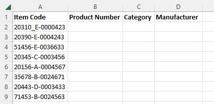
If we wanted to extract the product number located on the left side of this text, we could use the LEFT function to extract it. In each case, the product number is a fixed length, specifically five characters.
This means all we would need to do is enter the formula for the LEFT function:
=LEFT(cell reference, number of characters)
We will substitute the cell reference A2 and the number of characters, 5.

This will provide us with the extracted product number, and though we could enter the same formula substituting the correct cell references in the remaining cells, there is a quicker way.
Simply select the fill handle on the bottom-right of the cell with the formula we just ran and drag it down over the remaining rows.

Excel will apply the formula to each of the selected cells while automatically updating to the appropriate cell reference.
Extracting a Substring Using the MID Function
In order to extract a substring from a location within a given string, the MID function can be used.
This will begin extracting from a specified location within the string.
Following our example, we can extract the category code from within the item code by using the MID formula =MID(cell reference, starting location, number of characters).
Substituting our own cell reference of A2, the number of characters which is 7, and the number of characters to be extracted, 1, we have =MID(A2,7,1).
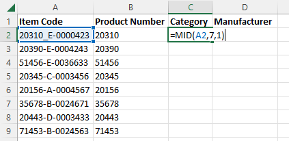
This will provide us with the category code, E, and the same as above.
The fill handle can be used to extend the formula to the remaining rows.

Extracting a Substring Using the Right Function
In the same way as the LEFT function extracts a set number of characters starting from the left side of a string, the RIGHT function extracts a certain number of characters starting from the right.
In order for us to extract the manufacturer code from our list of item codes, we will use the formula:
=RIGHT(cell reference, number of characters)
We will substitute our cell reference A2 and the number of characters seven and run the function.

This will provide our manufacturer code, and then we will use the fill handle to extend the formula to the remaining rows.

How To Use Text Functions To Extract a Substring Without a Fixed Length
These previous methods are great when working with substrings of a fixed length.
In this case, they are easy to use and do not require complex formulas; however, in many cases, you may be working with strings that are not as simple as this.
When the substrings you are working with are of variable lengths, these previous functions will not work because they require the input of an exact length.
However, by incorporating the SEARCH and Find functions into the formulas, we can still extract a substring.
These formulas will find and provide the numbers we need to provide the previous functions with the value they need.
These functions make it easy to extract data when the source cells contain uniform delimiters such as hyphens, commas, or spaces, which separate the substrings from the rest of the data.
Keep in mind that when deciding which of these functions to use with the extraction functions, SEARCH is not case-sensitive, but FIND is.
How To Extract Substrings Preceding or Following a Delimiter
You may notice that in each of the item codes we have been working with, the substrings are each separated by a hyphen.
This is convenient because we can use these symbols as a delimiter for Excel to determine what data to extract.
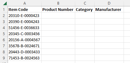
Though, in our case, the data has a hyphen. Excel does not require a delimiter to be any particular type of character.
You can even use a space as a delimiter to extract text. You simply need to find any uniform delimiters within the data you are working with.
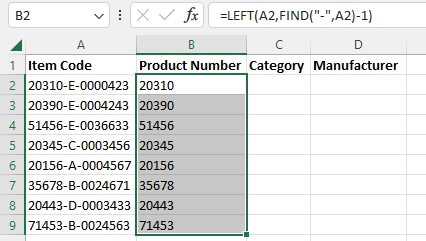
Now let’s say we wanted to extract the Product Number using the hyphen preceding the Category code as a delimiter.
We would use the formula:
=LEFT(A2,FIND(“-“,A2)-1)
We would substitute in our cell reference of A2, our “-” as the delimiter.
The FIND function within our formula will search for the first occurrence of the delimiter from the cell and return its position, and we subtract 1 from the resulting number of characters so that when Excel extracts the Product Number, it excludes the hyphen.

In our case, for example, the FIND function will return 6, which is the position of the first hyphen in our string.
Our formula will then subtract one for a total of 5 characters which the LEFT function will then extract into our cell.
We can then drag down the fill handle to extend this formula to the rest of the rows.
Now, because we have the same delimiter separating the category code from the manufacturer code and the FIND and SEARCH functions will only return the first occurrence of the delimiter, which is after the Product Number, we will have a slightly harder time extracting the other two pieces of data.
Because the category code is only one character in each case, we can use the following formula to extract the manufacturer code:
=RIGHT(A2,LEN(A2)-FIND(“-“,A2)-2)
This will subtract two characters from the result removing the category code and the hyphen, and similarly, we could extract the Category code using the LEFT function from the manufacturer code.
However, there will not always be a fixed number of characters to work with between the first and second instance of a delimiter.
This means that we need a new formula that can find the second instance of a delimiter and extract the text following it.
This substantially increases the complexity of the formula that must be used, but it is possible.
Extracting a Substring Occurring After a Pair of Delimiters
In our example, we have two hyphens separating the three substrings we want to extract. If we had two distinct delimiters, we could use the formula:
=RIGHT(cell reference,FIND(“delimiter”,cell reference)-1)
However, because they are the same symbol and the FIND function will only return the first instance of a symbol, we will need to use this formula:
=TRIM(MID(cell reference,FIND(“#”,SUBSTITUTE(cell reference,”delimiter”,”#”,occurrence))+1,100))
As you can see, you are not limited to only the second occurrence of the symbol either, and can, in fact, substitute the third, fourth, or any occurrence of the symbol. In our case, we will substitute A2 for the cell reference and “2” for the occurrence and enter it in our blank cell.

This will return the Manufacturer code in the first row, and we can use the fill handle to drag down and extend the formula to the remaining rows providing us with all of the Manufacturer codes.

Extracting a Substring from Between a Pair of Delimiters
Now we need to extract the Category code, which is located between the two delimiters. To do this, we will use the formula:
=SUBSTITUTE(MID(SUBSTITUTE(“delimiter” & cell reference&REPT(” “,6),”delimiter”,REPT(“,”,255)),2*255,255),”,”,””)
We will substitute our cell reference and delimiter into the formula and enter it in a blank cell. Once run, this will provide us with the Category code located between the two hyphens.

As with the previous formulas, we will drag down the fill handle and extend the formula to the rest of the rows.

As you can see, it is possible to extract substrings occurring before, after, or between delimiters regardless of fixed length. Though these functions are extremely flexible and dynamic, meaning the results will update with changes in the source data, they can be difficult to work with.
Depending on the length, uniformity, and type of delimiters, the formulas required can become extremely complex. Adapting these text functions to your needs can require considerable skill in some situations.
Fortunately, there is an easier way to extract a substring in some cases using one of Excel’s built-in features.
Extracting a Substring with Excel’s Text to Columns Feature
As we have seen, text functions are a powerful tool, but they can quickly become extremely complex.
For situations where you do not need your substring to update with changes in the source data, Excel’s Text to Columns feature can often provide a much simpler alternative to using text functions.
This tool can extract text based on delimiters located in text strings, similar to using text functions.
However, you can complete the entire process within the “Convert Text to Columns Wizard,” making it easy to do without needing to enter any formulas.
Simply follow these steps:

- Select all of the cells containing the substrings you want to extract.
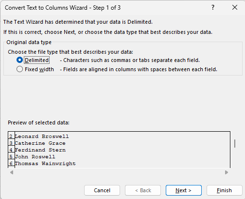
- Navigate to the “Data” tab, and within the “Data Tools” group, select “Text to Columns,” and the “Convert Text to Columns Wizard” will open.
- In Step 1 of the Wizard ” select “Delimited” under “Choose the file type that best describes your data” and select “Next.”

- In Step 2, you will select the type of delimiter that is present in your string, and Excel includes default options for the most common delimiters. If yours is present, place a check in the box next to it or select “Other” and enter the appropriate delimiter in the box to the right. Excel will display a preview of how your data will be split below. Confirm that this looks correct and click “Next.”

- Step 3 of the wizard will ask how you want your data to be formatted, and if it is text, then either the “General” or “Text” format will work just fine. If you are extracting a number or date, then change the format selection appropriately. You can also choose the destination cell, which by default, will be the location of the original data. If you would like to retain the original data, then change this to another location.
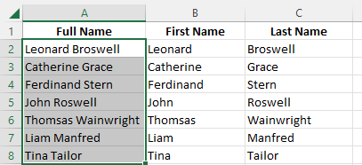
- Click Finish, and the “Convert Text to Columns Wizard” will extract the data into two substrings located in your chosen cells.
As you can see, this process is extremely simple compared to using text functions.
In addition, if you need to further split the text, you can repeat the same process as many times as you need.
Conclusion
Now you know how to use Excel’s text functions to extract substrings in a variety of circumstances.
Though this can require a bit of skill to adapt to each situation, they are truly a powerful and dynamic tool.
In circumstances where data is formatted more simply, and the source data does not need to be regularly updated, Text to Columns can be an easier-to-use alternative to extract a substring.
