How to Compare Two Columns in Excel (Using VLOOKUP & IF)Step by Step Guide with Screenshots


Working with Excel, especially with large amounts of data, could mean that you will need to compare data sooner rather than later.
With small data, it is easy to spot similarities or differences.
But dealing with a large amount of information can be a challenge.
This Excel article will provide the different methods of comparing two columns and finding their matches and differences.
The methods used include the VLOOKUP Formula, IF Formula, or Conditional Formatting.
Side-by-Side Comparison of Two Columns
Probably the most basic method of comparing two tables is to look at the data in one table and compare it with the other.
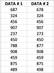
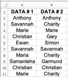
If you wish to check whether the data in Column A versus the data in Column B is the same or not, let’s take the below table as an example.
Manually entering data poses a higher chance of human error.
This cannot be avoided.
However, there are simple ways of spotting differences in Excel using the different methods which will be illustrated in the next sections below.
Using the Equal to Sign Operator
Based on the example above, you wish to see which of the columns have matching or non-matching data.
The simplest formula to do this is shown as =A2=B2.
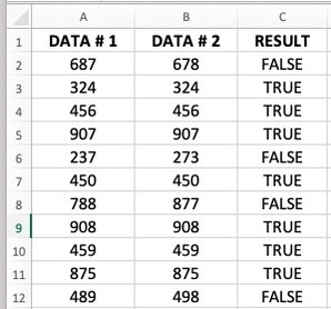
If the data in Column A and Column B are the same, the result shows as TRUE.
Otherwise, it shows as FALSE.
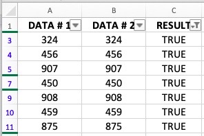
If you wish to see only the data that match or do not match, you can use the filter option.
Using the IF Function
Apart from the equal sign, the IF function can also be used to find similarities and differences when comparing two columns.
It functions just the same as when using the equal sign with one profound difference: you will be able to decide the value to get when it comes to the resulting similarities or differences.
For example, you can decide for the result to show as “Match” for similarities and “Mismatch” for differences.
The formula to be used is:
Use the formula `=IF(A2=B2,”Match”,”Not a Match”)` to quickly compare the values in cells A2 and B2. If the two cells contain the same value, Excel returns “Match”; if they’re different, it returns “Not a Match.”
The result would show as follows:
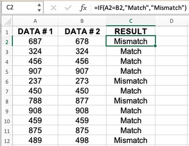
Evidently, the IF function and equal sign operator basically have the same formula.
However, since we are using the IF function, we can ask the equation to return a specific value.
Highlight Rows with Matching Data (or Different Data)
Other than the two methods shown above, another method to use is conditional formatting.
And in such a case, you have the option to highlight values that are different and the same.
Suppose you wish to determine whether names have been duplicated in each column.
Take the table below as an example:
You can follow the steps below to proceed with conditional formatting:
- Select the data to be formatted.
- On the Home Tab, under Styles, select Conditional Formatting.
- Click on New Rules > Use a formula to determine which cells to format.
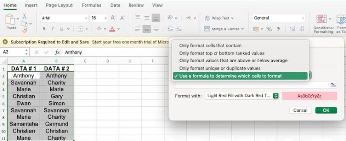

- Supply this formula in the tab: =$A2=$B2. Under Format With, select the type of formatting that you wish to use. Click on OK.
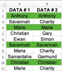
- The result will be shown below.
If in case you wish to only highlight the rows that are different, you may do so by using the below formula:
=A2<>B2
Comparing Two Columns Using VLOOKUP
Using VLOOKUP (Find Matching/Different Data)
When your data is a bit more complicated and you need something more than an equal to function, the best solution for that would be to use VLOOKUP.
This is important when you need to determine if there exists a data point in one column compared to another column.
Using VLOOKUP and Find Matches
Suppose you wish to see if the data in Column A also exists in Column B, you can use the VLOOKUP formula below:
=IFERROR(VLOOKUP(B2,$A$2:$A$11,1,0),”No Match”)
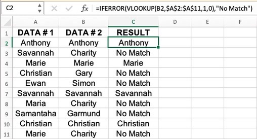
The result above shows the name in Column C if it is a match and returns No Match if the data in Column A and Column B are not the same.
Using VLOOKUP and Find Differences (Missing Data Points)
Using the example above, you can use VLOOKUP to check data in Column B that are not found in Column A.
We can use this formula to do just that:
=IF(ISERROR(VLOOKUP(B2,$A$2:$A$11,1,0)),”Not Available”,”Available”)

The above formula will return “available” if the names in Column B can also be found in Column A.
If there is no match, it returns “not available”.