Filtering Data in an Excel Pivot TableThis tutorial will show you the different filters that can be done based on different data types


Excel provides many options when it comes to filtering data in a Pivot Table.
This tutorial will show you the different filters that can be done based on different data types.
Pivot Table Filter Types
Shown below are the different filter options available for your Pivot Table on Microsoft Excel:

Here are what the filter types mean:
- Report – Drag and drop the heading to the Filters side of the Pivot Table editing pane. In the example above, the Market is in the Reports filter, meaning that data analysis can be done for each market or several markets, depending on your selection.
- Row or Column – Using this filter, the data can further be filtered according to text or values.
- Search Box – This can be done using the row or label filter. As an example, suppose you want to filter only the sales made by a specific salesperson, simply type the name on the search box and tick on the box when the search result shows. The Pivot Table will then show all of the relevant data for that person.
- Check Box – Select the result or results that show. Once selected, you will be able to see all the pertinent information already filtered for the specific information chosen.
Examples of Filters Used in Pivot Tables
There are many ways to use the filter option in Pivot Table. Some of them included the following:
- Filter by Value, Percent, or Sum of the Top or Bottom Items
- Filter by the Specified Percent of the Value of the Top or Bottom Items
- Filter by a Specified Value the Top or Bottom Items
- Filter by Search Box
Top 10 Items Filter
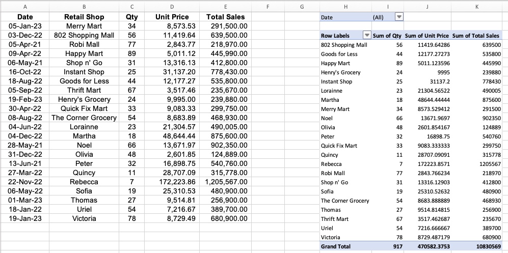
Let us take the data below as an example:
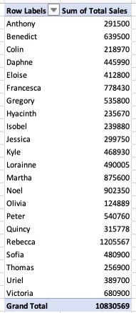
Using the above information, let us try and filter the data into the top 10 items.
Filter by Value, Percent, or Sum of the Top or Bottom Items
Using this filter, we will be able to ascertain the top 10 or bottom 10 salespersons by total sales value.
To do this, simply follow the steps below:
- Click on the filter for the row label.
- Hover over Value Filters.
- Select Top 10.
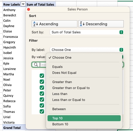

When you click on Top 10, you will encounter 3 options to choose from.
They are the following:
- Suppose you are looking for the top 10 salespersons, select Top 10.
- Even if you are looking for the Top 10, you can still select the number of items you actually need. In this case, set it at 10.
- You can then select which among these three options you need: Percent, Items, or Sum. For the purposes of this example, choose Item.

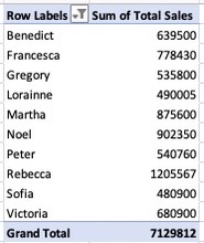
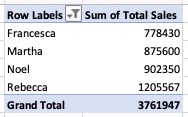
Based on the filter selected, you will have the below data:
If you wish to view the bottom 10 of your dataset, you can choose the Bottom 10 instead of the Top 10 and follow the same process.
Filter by the Specified Percent of the Value of the Top or Bottom Items
Following the same example above, let’s say you want to filter by percent instead of items. The steps will still be the same as follows:
- Click on the filter for the row label.
- Hover over Value Filters.
- Select Top 10.
- Suppose you are looking for the top 30% of the total sales by salesperson, select Top 10.
- Select 30.
- Choose Percent.
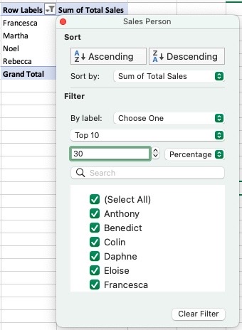
You will get the below result:
If you wish to view the bottom 30% of your dataset, you can choose the Bottom 10 instead of the Top 10 and follow the same process.
Filter by a Specified Value the Top or Bottom Items
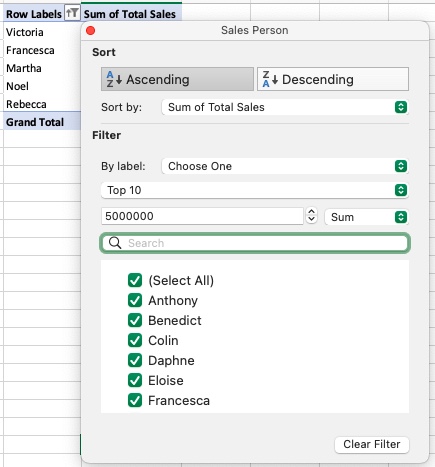
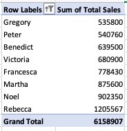
Still using the same steps above, you can also filter by determining the top salespersons that makeup $5,000,000 in sales. Here’s how you can do this:
- Click on the filter for the row label.
- Hover over Value Filters.
- Select Top 10.
- Enter the value 5000000.
- Choose Sum.
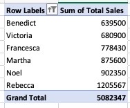
Based on the filter options above, here is what the result will be:
Value Filter on Items
Another filter option would be to see only specific values using the same example above.
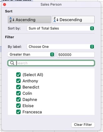
Suppose you wish to filter only the salespersons who made $500,000 in sales and above, here are the steps to do it:
- Click on the filter for the row label.
- Hover over Value Filters.
- Choose Greater Than. There are also other filter options such as Less Than, Does Not Equal, etc.
- Input the value you wish to filter. In this case, it is $500,000.
You will get the result below:
Cell Value Filter
To filter a pivot table using a specific value, we may need the help of a VBA Code which we will be showing in the next section.
Simply follow these steps:
- Choose the cell you wish to enter the Pivot Table in. In the below example, I chose cell H1.


- Right-click on the excel tab that contains the Pivot Table and Click on “View Code”.
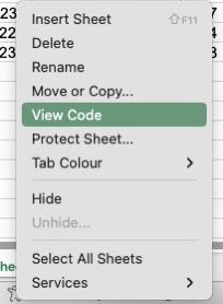

- Copy the code below to the VBA Code Window to filter by Cell Value:
Private Sub Worksheet_Change(ByVal Target As Range)

'Update by Extendoffice 20180702

Dim xPTable As PivotTable

Dim xPFile As PivotField

Dim xStr As String

On Error Resume Next

If Intersect(Target, Range("H6:H7")) Is Nothing Then Exit Sub Application.ScreenUpdating = False

Set xPTable = Worksheets("Sheet1").PivotTables("PivotTable2")

Set xPFile = xPTable.PivotFields("Category")

xStr = Target.Text

xPFile.ClearAllFilters

xPFile.CurrentPage = xStr

Application.ScreenUpdating = True

End Sub
Here are some of the notes you need to consider:
- The worksheet is referred to as “Sheet 1”.
- The Pivot Table has the name “PivotTable2”.
- “Category” is the name of the pivot table’s filtering field.
- Cell H1 contains the value you wish to use to filter the pivot table.
The filter will then be shown as:
Label Filters on Data
When you work with huge chunks of information, using Label Filters is an excellent idea to save you a lot of time.
Take the below data as an example:
Here’s what you need to do to execute the Label Filter:
- Click on the Row Label Filter.
- Select Label Filter.
- Click “Contains”.
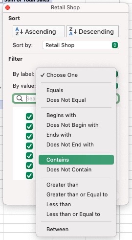

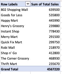
- For the purposes of this example, suppose you wish to see the retail shops that only contain the name “mart”. Type this in.
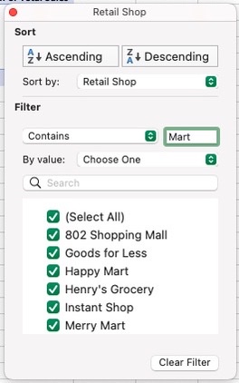

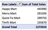
You will get the result below:
Note: There is no option to add more words in the search box as this does not have additive criteria. The latest character you type will be the resulting data.
Search Box Filter on Data
This works similarly to filtering by label except that you can proceed to immediately use the search box.
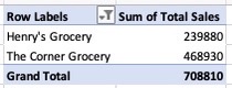
For example, you only want to see the cells that contain “Grocery”. Type this in the search box as shown below:
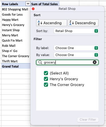
This will immediately filter and show only the cells that contain grocery in the name.
The result of this search will be:
Here are some of the notes that you need to consider when using the search box:
- The first criterion is disregarded and you obtain a list of the second criteria if you filter once with one and then again with another. There is no additive filtering.
- You will be able to manually eliminate a few results when using the search box. For instance, you may perform a search for the word “bank” if you have a long list of financial organizations and just want to filter out banks. You may just uncheck and keep it out if any of the businesses entered are not banks and still show in the result.
- You can’t eliminate particular outcomes. There is no option to use the search box to filter only the merchants that have the word dollar in them, for instance. Nevertheless, you may do this by utilizing the filter “does not contain” option.