A Simple Guide to Creating Excel Dynamic Chart TitlesEasy Tutorial with Screenshots
A lot of times, when we create charts, we miss out on changing the chart’s title and it ends up with the label “Chart Title”.
We would not want our work not to have a proper chart title now, would we?
So let’s begin and delve into the topic of creating dynamic chart titles in the section below.
Cell Value Linking
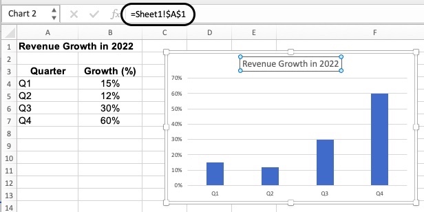
Take the below image as an example:

To change the Chart Title as shown above, it has to be manually done each time the table is refreshed or updated because this data is static.
There is, however, a way to make it more dynamic so you don’t have to manually change it and forget to do so the next time you update the table. Here are the steps to do it:
- Hover over Chart Title and click on the box.
- Type “=” on the Formula Bar.
- Click on the cell you want the Chart Title to show as.
- Click on Enter.
The Chart Title will now show as:

Combination of Cell Link & Text
Let’s say you want the title to be more than the value of the cell you have linked like the one above, and you want to add text.
You can do this by creating a formula for another cell.
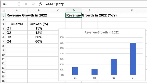
For example, you wish to add “YoY” to the title.
Follow these steps to achieve this:
- Click on a new cell and type “=”
- Click on the cell you want your chart title to show as.
- Add this in the formula bar: &“ (YoY)”

- With the new formula, click on the Chart Title box and type “=”
- Click on the cell with the new formula.

Conclusion
The steps we have shown above are incredibly simple to execute and will save you a lot of type from manually changing chart titles.
This will also ensure that you don’t miss changing this each time you update your chart.


