Deleting Filtered Rows (With & Without VBA) in Microsoft ExcelStep by Step Instructions with Screenshots
There are a lot of functionalities present in Excel.
A lot of users do not even know how to use all these functionalities.
Among the features that are present in Excel are filters.
This is one way of hiding unnecessary data that you need.
You can view only the data that you need to see while keeping irrelevant rows hidden.
This way, you can focus on the data that you are working on without the unnecessary word/text in your spreadsheet.
You can also delete the irrelevant rows if you don’t need them.
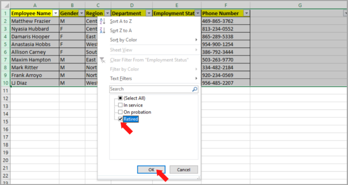
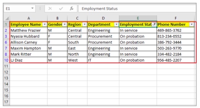
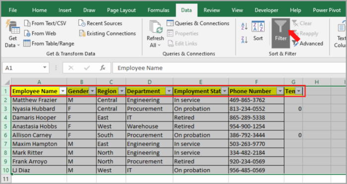
Here is our sample datasheet as shown in the image below.
These are records about the company’s employees.
Here you can see the status of the employee (retired, in service, and on probation).

In this sample data, you might not need the information of the employees that are already retired. Therefore, you might delete the rows that contain the data of the retired employees.
In Excel, you can automatically delete the rows that have a retired status on them.
By using filters, you can delete them with ease. In this tutorial, we will show you how these filters are properly used, and how you can delete filtered rows in Excel.
We will tackle how to delete visible and invisible rows with filters on them.
If you are comfortable with coding and like to speed up your work, you can use VBA code in Excel.
How to Delete Visible Filtered Rows?
Here is how you can use a filter on the rows and delete them:
- Select all the data in your worksheet.

- Go to the Data tab and click the Filter button (in the Sort and Filter group).

- In the header row, you can see that an arrow will appear. Click on the arrow and select the filter that you need.

- For example, we need to filter only the rows that have the “Retired” employee status. Click the arrow beside the “Employment status”, and uncheck all of them, except the “Retired” status.

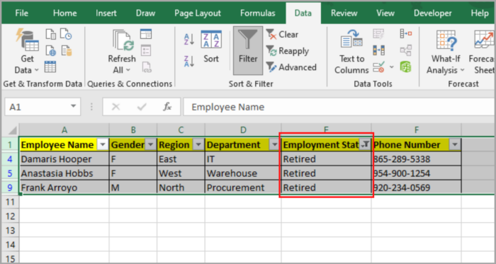
- Click the OK button and you will only see the rows that have “Retired”.

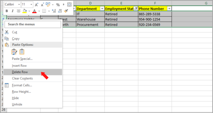
- You can now safely delete the “Retired” employee. Don’t worry, this action will only delete the visible rows and the rest will be safe.

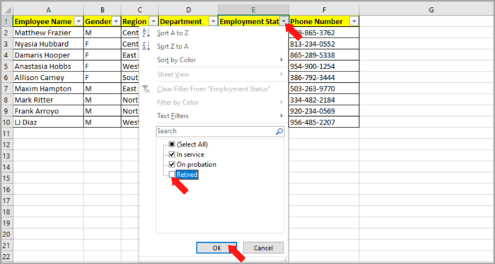
- If you want to see all the data, you can simply click on the Filter button located in the ‘Data’ tab.
After doing this step-by-step method you can now see all your data, without the Retired employees.

How to Delete Visible Filtered Rows by Using VBA?
VBA coding is very intimidating, especially for basic users of Excel. But you can use VBA coding by simply performing copy-and-paste actions in Excel.
You can copy this script and paste it:
Sub DeleteVisibleRows() Dim Rng As Range Set Rng = Selection Rng.AutoFilter Field:=5, Criteria1:="Retired" Rng.Offset(1, 0).SpecialCells(xlCellTypeVisible).EntireRow.Delete ActiveSheet.AutoFilterMode = False End Sub |
- This is an ‘Autofilter’ depending on your filtering criteria (line 4). This is to make sure that the row will only appear with the criteria you want.
| Rng.AutoFilter Field:=5, Criteria1:=”Retired” |
- In Line 5, this line will automatically delete the visible rows (Retired).
| Rng.Offset(1, 0).SpecialCells(xlCellTypeVisible).EntireRow.Delete |
- Lastly, it will get rid of the filters by setting up the spreadsheet’s AutofilterMode to False (line 6).
| ActiveSheet.AutoFilterMode = False |
Here are the steps for using the given code above:
- In your spreadsheet, select all the rows you want to filter. This will also include their column header.
- Go to the Developer Menu ribbon, and select Visual Basic.
- The VBA window will now be opened, go to Insert > Module and in your Module window paste the given code above.
- Lastly, Run the code by going to Developer>Macros>DeleteVisibleRows or you can click the play button (green) from the toolbar above.
Note:
You can insert any word/text to fit your criteria. You can replace the word “Retired” with In service etc.
How to Delete Hidden Filtered Rows?
Let us go to a more complex example of using our filter.
We are going to use the employees that are in service or on probation.
If you have a complex filter, the program would prefer to delete the rows that don’t suit the description rather than those that do.
In this case, the program will prefer to delete the rows that are hidden after using the filter.
We are going to use the dataset that we used earlier. In this problem, we are using two filters – the first filter is to remove rows with the word “Retired” and the other is to remove the row that doesn’t contain “Procurement”.
Here are the steps for using the given code above:
- In your spreadsheet, select all the rows you want to filter, which can also include their column header.
- Go to the Data tab, and click the Filter button (located in the ‘Sort and Filter’ group).

- Click the filter arrow (Employment Status header) and uncheck the box next to “Retired”.

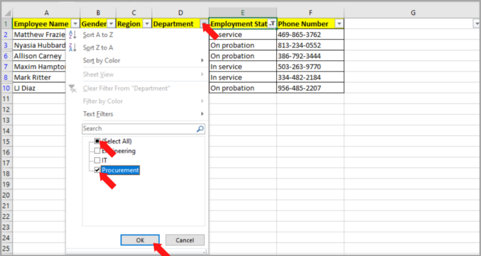
- Then, click the Filter arrow (Department header) and uncheck all the boxes except “Procurement”.

- Lastly, click the OK button. You will now only see the rows with Employment Status “In service” or “on probation” and Department “Procurement”.

To delete the hidden rows, there are three ways to do this.
How to Delete Rows that are Hidden By Using the Feature Inspect Document
If you are certain that you are not working with the hidden data, this method will be helpful in your work.
Here is the step-by-step process of this method:
- Back up your workbook (just in case).
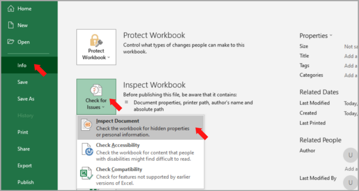
- Go to File>Check for issues.
- Click on Inspect Document.

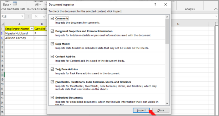
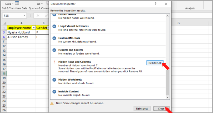
- The ‘Document Inspector’ will be opened. Now, click on the ‘Inspect’ button located at the lower right side of the window.

- There is an option that says ‘Hidden Rows and Columns’ when you scroll down the list. This also tells you how many hidden files are present in your spreadsheet.
- You will see “Remove All”. Click it – this action will permanently delete all the hidden rows in your spreadsheet.
- Click the ‘Close’ button.

- To remove all filters, go to the Data Tab and click on the filters. Go back to your worksheet.
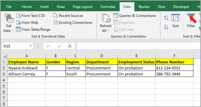
You are now left with only your relevant rows for your project and all the rows that you don’t need are now permanently deleted.
How to Delete Rows that are Hidden By Temporary Columns
If you don’t want to back up your data and don’t want to make permanent changes to your worksheet, here is another way to delete these hidden rows:
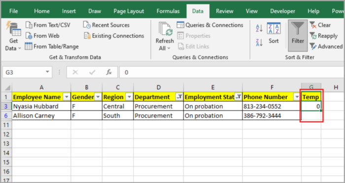
- Anywhere in your worksheet, create a temporary column.

- In the first cell of the column you created, type zero (0) and press the Enter key.

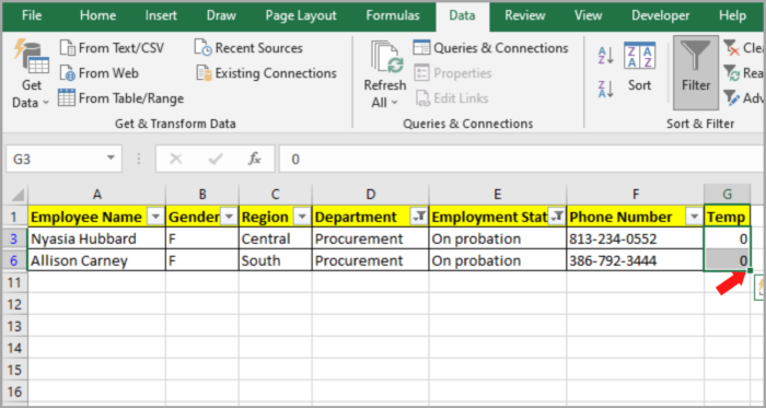
- Copy the zero (0) to the rest of the cells in the column by dragging down the fill handle in the cell.

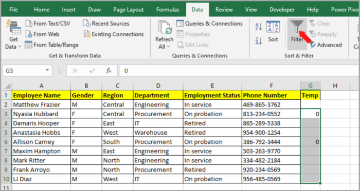
- By clicking the Filter button from the Data tab, remove the filter (this action will bring back all the hidden rows).

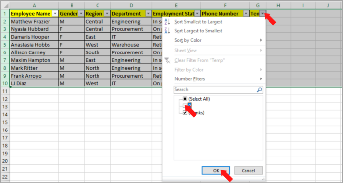
- We need to reverse the filter. Select your entire work area and click on the Filter button. Uncheck the box beside zero (0) by clicking the arrow next to the header of the temporary column you created.

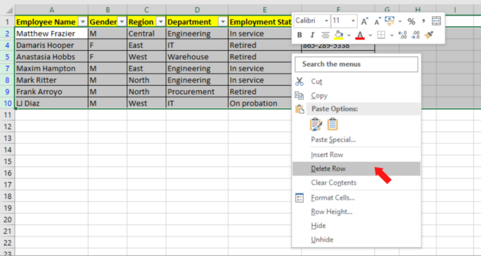
- Just select all the rows and ‘Delete’ them.

- Remove the filter again by clicking on the Filter button.

You are now left with only the relevant rows for your project while all the rows that you don’t need are now permanently deleted.
How to Delete Hidden Filtered Rows By Using VBA
We are again using code to delete the hidden filtered rows.
Here is the code that we will be using:
Sub KeepVisibleRows() Dim myUnion As Range Dim myRow As Range Dim Rng As Range Set Rng = Selection Rng.AutoFilter Field:=4, Criteria1:="Sales" Rng.AutoFilter Field:=5, Criteria1:="<>Retired" ForEach myRow In Rng.Rows If myRow.Hidden Then If Not myUnion IsNothingThen Set myUnion = Union(myUnion, myRow) Else Set myUnion = myRow EndIf EndIf Next myUnion.Delete ActiveSheet.AutoFilterMode = False End Sub |
Here is the step-by-step process for using this code:
- In your spreadsheet, select all the rows you want to filter. This also includes their column header.
- Go to the Developer Menu Ribbon, and then select Visual Basic.
- The VBA window will now be opened. Go to Insert > Module and in your Module window paste the given code above.
- Lastly, Run the code by going to Developer>Macros>KeepVisibleRows or you can click the play button (green) from the toolbar above.
Here is how the code works:
- This code selects the rows and applies ‘AutoFilter’ to them according to the word you want (in line 6 and line 7).
| Rng.AutoFilter Field:=4, Criteria1:=”Sales”
Rng.AutoFilter Field:=5, Criteria1:=”<>Retired” |
- You can see that in line 6, we want to display the rows with only the word “Sales” (column 4).
| Rng.AutoFilter Field:=4, Criteria1:=”Sales” |
- Also in line 7, we want to display the rows only with Employment Status not equal to “Retired” (Column 5).
| Rng.AutoFilter Field:=5, Criteria1:=”<>Retired” |
- The two lines mentioned above make sure that the criteria that we are looking for will be shown, while the other selection will still be hidden.
- Then, the code reads along every row and verifies for possible hidden cells. In our example, it is line 9.
| If myRow.Hidden Then |
- If that is the case, they will be added temporarily within a range called “myUnion”. If every row was read, all the rows that are hidden will be grouped together to myUnion.
| Set myUnion = Union(myUnion, myRow) |
- When the looping or reading is done, every row that is added in myUnion will be removed. Here, it is line 17. Meaning, every hidden row will be removed at once.
| myUnion.Delete |
- Lastly, the filter will then be removed by programming the excel sheet to False (from AutoFilterMode). Here, it is line 18.
| ActiveSheet.AutoFilterMode = False |
Note: As aforementioned, the 6th and 7th lines can be altered to match your preferred filter categories or criteria.
If you have more than one category, you can repeat these lines for each category.
Conclusion
In this article, we illustrated two methods for deleting the rows that are visible and three methods for deleting the rows that are hidden.
Moreover, we also gave short VBA codes to help you finish your tasks faster.
We hope you followed the steps quickly and found this article useful.


