Creating a Drop Down Filter to Extract Data Based on SelectionTutorial with Screenshots


Excel is an amazing application for storing data for future use.
However, when referencing large quantities of data, it can become cumbersome to sort through data by hand.
By using a drop-down filter, it is possible to filter and extract data based on selection.
For example, with a drop-down list, it is possible to select one item from a drop-down list, and the associated rows for the selection will be extracted.
This can greatly accelerate the process of referencing information contained within a database.
Here we will take a look at how you can filter data using a drop-down list.
How To Extract Data Using a Drop-Down List in Excel
To extract data based on the selection using a drop-down list, there are a few different steps you will need to follow.
This includes creating a list of unique items from which the drop-down list will pull, adding a drop-down filter, and creating helper columns to help Excel sort the data.
By following these steps, we can allow Excel to identify and extract information based on our selection in the drop-down filter.
So, let’s take a closer look at how to complete this process, starting with preparing the dataset.
Create a Unique List
Not every item in a dataset may be completely unique, but in order to differentiate selections, you will need a unique identifier in order to select them from your drop-down list.
So, your first step will need to be ensuring your filter selections are ready by ensuring you have a unique identifier for each item in your dataset.
Here is a simple way to do this.
- Select and copy the cells containing the items you would like to use as identifiers for your drop-down list and paste them into another section of your spreadsheet.

- Navigate to the “Data” tab, and within the” Data Tools” group, select “Remove Duplicates.”

- This will open the “Remove Duplicates” screen, which will contain all of the selected items while removing duplicates. This is the list of selections you can use to create your drop-down list.
Inserting a Drop-Down List
Now that the unique dataset you will use for your drop-down list is ready, it is time to insert it into a cell.
Simply follow these steps.
- Navigate to the “Data” tab, and from the “Data Tools” group, select “Data Validation.”

- This will open the “Data Validation” screen, where you can navigate to the “Settings” tab.
- Here from the “Allow:” selection, choose “List,” and for “Source:” select the unique data set you created in the last step.

- With the data selected, click “OK.”
Now that your drop-down list is created, it is time to prepare your data set for the filter to extract your desired data.
Creating Helper Columns
In order for your drop-down filter to make selections from your dataset, we will need to provide it with a way to identify your desired selections.
To do this, we will use helper columns, and here is how to insert them into your worksheet.
- Create the first helper column you will need by entering a serial number for each record.

- Enter the formula =IF(A2=$H$2,D2,””) into the topmost cell of the next column and use the fill handle to drag down and extend it to the remaining cells in the column. This formula will check for a match against the cells containing the drop-down value, and if it is discovered, it will return the row number or a blank.

- Now we need a way to extract the data for rows that return a number, and to do this; we can create a third helper column. In the next column, over-enter the formula and once again use the fill handle to extend it to the other cells in the column.
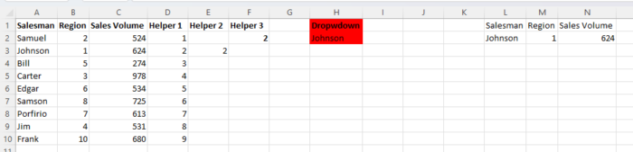
Adding an Output
Once You are finished adding helper columns, it can be a good idea to prepare a space for the selected data to be displayed.
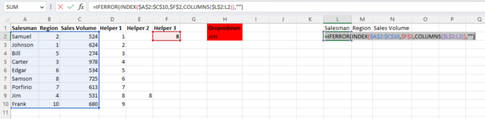
Choose a cell, in our case L2, and enter the following formula =IFERROR(INDEX($B$4:$D$23,$G4,COLUMNS($J$3:J3)),””) and drag to extend it as far as you need to contain your results.
This will allow the filtered data to be outputted correctly.
Finish Up
Now your drop-down list should be fully functional, and you can go ahead and hide the original dataset if you would prefer.
This can be useful for extracting data when it is needed without leaving your worksheet looking cluttered.
Whichever you choose, your drop-down filter is guaranteed to leave the process of filtering and extracting much more efficient.