Convert Text to Numbers in ExcelA Step By Step Tutorial


If you work in Excel often, chances are you will find numbers that are formatted as text in Excel.
These characters may look like numbers, but when it comes to using them in formulas, they just won’t add up right, causing errors.
In most cases, Excel will convert numerical strings into numbers automatically when spreadsheets are imported; however, when it fails to, or numbers are incorrectly formatted as text when numeric data is entered, it can greatly impact the outcome of calculations.
This is because when incorrectly formatted as text, Excel will not recognize your numeric data as a number causing it to return errors or incorrect results.
Fortunately, Excel provides several ways that you can convert text into numbers saving you valuable time and ensuring you have the accurate data you need.
Why Numbers Become Stored as Text
Before learning how to identify and convert text into numbers, it is important to understand the most common reasons that numbers become formatted as text in the first place.
This will help you to avoid this occurring in the future.
- An apostrophe is placed before a number. Many users will include an apostrophe before numbers in order to force spreadsheeting software to treat it as a number. This may be done for various reasons; however, when it comes to using these numbers for data, it is a big problem. This often may be encountered when numbers are downloaded from a database, in which case the apostrophes may not be present, but the numbers will still be treated as text.
- Numbers generated from formulas such as MID, RIGHT, OR LEFT. If a number is acquired from a text string with the TEXT function applied, then it will remain in text format unless it is converted into a number.
How To Identify Numbers Formatted as Text
Excel includes a built-in feature that checks for potential issues with cell values and provides warnings.

This will appear as a green triangle at the top-left of a cell.
Once a cell with an error message is selected, Excel will bring up a caution sign.
By hovering over the sign, you can see the error message, which, if the number is formatted as text, will be: “The number in this cell is formatted as text or preceded by an apostrophe.”
Excel may not always display this message when numbers are formatted as text, but there are other ways to tell.
Perhaps the easiest is that correctly formatted numbers will always be right-aligned by default, whereas text is left-aligned.
In addition, when multiple cells containing numbers are selected, the status bar will display Average, Count, and SUM, whereas, in the same situation, the text will only display Count.
Finally, numbers formatted as text will often have an apostrophe preceding them in the formula bar.
Convert To Text Number Format on the Home Tab

For a small number of cells, the easiest way to convert text into a number format is to do it manually through the “Home” tab.
You can do this by selecting the cell containing the text and, within the “Number” group, clicking on the arrow to bring up a drop-down menu with formatting options.
This will contain several formatting options, including “General,” “Currency,” and “Accounting,” among others.
However, we will select “Number” from the list to change the formatting to a general number format.
You could alternatively choose the “General” format instead, and this will typically present a few problems.
The difference is primarily that it will limit the size of numbers by rounding large decimal values and using scientific notation for numbers with more than 12 digits.
Convert Text to Numbers with the “Text to Columns” Button
One of the easiest ways to convert text to numbers is with Excel’s “Text to Columns” feature.
This feature is normally used to separate values into multiple distinct columns; however, it is also one of the easiest ways to convert formatting in Excel. Here is how:
- Select the cells or columns that you would like to convert. This can include an entire column of data or simply a range of cells.
- Select the “Text to Columns” button. This is located in the ribbon under the “Data” tab inside of the “Data Tools” group.
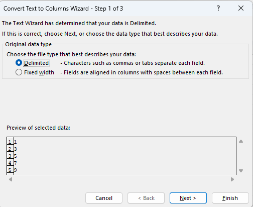
- Simply select “Apply” or “Finish,” depending on your version of Excel. Unless you have a reason to separate your data into separate columns, you do not need to navigate through the many options offered by the “Convert Text to Columns Wizard.” Either elect “Finish” as soon as the wizard opens or select “Next” through every step without making any changes and select Finish at the end.
Once the wizard is complete, it will set all of the contents to Excel’s “General” format, which means that numerical values will be converted into the “Number” format, dates will be set to the “Date” format, and text will be set to the “Text” format.
Use Excel’s Error Message to Reformat as a Number

When Excel recognizes that numerical values may have been formatted as text in error, it will place a warning message to alert you.
By using this message, you can quickly reformat numerical values into text.
When you hover your cursor over the error message, it will explain the error, and by selecting the arrow next to it, you can open a drop-down menu with options relating to the error.
This includes “Convert to Number,” and by selecting this, Excel will reformat the cell to text, solving the problem.
Use the VALUE Function to Convert Text to Numbers
The VALUE function can be used to copy data into a new column while simultaneously converting it into a number format.
This can be a convenient way to convert a large number of cells at once with a formula, which can often be faster than using the ribbon tools for experienced users. Here is how.
- Insert an empty column. If there is already an empty column next to your data, that’s great! Otherwise, insert an empty column by right-clicking to the right of the column holding your data and selecting “Insert” to add a new column.
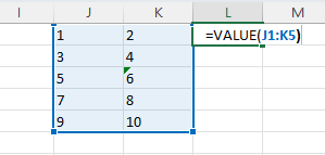
- Enter the VALUE function. In the top cell of the new column, or next to the top, if a column header is present, enter the formula: “=VALUE(Starting Cell:Ending Cell)“, substituting your own cell references for the starting and ending cells of the column.
- Run the formula, and Excel will copy the data into the new column and convert it into the correct format. You can now delete or otherwise deal with the old column of data as you choose.
As you can see, this is extremely easy to do. If you prefer using the fill handle instead of entering a starting and ending cell reference, you can do this as well.
Simply run the formula “=VALUE(Cell Reference” substituting the topmost cell in your column, and drag down the fill handle until you have highlighted every cell you want to convert.
Using Paste Special to Convert Text To Numbers
The previous methods work extremely well when converting single cells or columns; however, they can prove cumbersome when values in many different cells or columns are involved.
Fortunately, when this is the case, Excel’s “Paste Special” tool can work to convert text contained in many different columns. Simply follow these steps.
- Select a blank cell and enter the number 1. Make sure that the cell is formatted as “Number” or “General,” not “Text,” and press “Enter” on your keyboard.
- Select to copy the cell. You can use the “Ctrl + C” shortcut or right-click on the cell and select “Copy.”
- Select all of the cells you wish to convert into “Number” format. Keep in mind that this will change the formatting of incorrectly formatted numerical values, but it will not work for functions or numbers that are formatted as words such as “one.”
- Select “Paste” and then “Paste Special” from the drop-down menu. Navigate to the “Home” tab, and the “Paste” button can be found near the left-hand side of the ribbon. From there, the “Paste Special” option can be found on the drop-down menu.
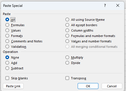
- Select “Multiply” to convert cell values to that of the copied cells. In the “Paste Special” dialog box, you can leave the “Paste” setting to all, and under “Operation,” choose “Multiply” before selecting “OK.”
- Excel will then multiply all your chosen values by “1,” providing you with the same values in the copied cells format. Now that your cells are all in the correct format, you can feel free to delete the number “1” you placed in the empty cell earlier.
Conclusion
Excel provides many ways to format and store data for a wide range of purposes, and as useful as this can be, it may also lead to difficulty using numerical data when it is incorrectly formatted.
Fortunately, you can use any of the methods above to easily reformat your data as numbers making it easy to perform calculations and allowing Excel to interpret and use numerical data free of errors.