How To Convert Multiple Rows to Single Row in Excel5 Simple Methods

Written By:
Lisa Borga

Excel is often used to store large amounts of data, and typically this means dealing with a correspondingly large amount of rows and columns.

Sorting through this data can be quite a hassle, let alone understanding it.

One thing that can often help is reducing the number of either rows or columns to give us an easier visual format for viewing the data.

Though manually converting data into a single row can be quite the hassle, here we will show you a few different easy techniques you can follow to convert multiple rows into just one.

So, let’s take a look!

Method #1 – Using the Transpose Function

As an example, let’s assume that we want to convert five rows containing our sales regions into a single row.

Using Excel’s TRANSPOSE function, we can do just this. The syntax for this function is:

=TRANSPOSE(RANGE)

Keep in mind that you do not need to manually enter your cell range.

After you enter” =TRANSPOSE(“, you can simply click and drag to select your range.

When you are finished selecting, click CTRL+SHIFT+ENTER on your keyboard to finish selecting.

Simply enter the formula into a blank cell where you would like your new row to be placed, select your range, and run the formula.

The TRANSPOSE function will convert your data from multiple rows into a single row.

As you can see, this is a really quick and simple method for turning numerous rows into just one.

Method #2 – Using the Power Query Tool

The Power Query tool is another method we can use to convert multiple rows into a single one, and we can access this tool right from the ribbon.

This is great for users who are less familiar or comfortable with using Excel’s functions.

Here are the steps we can follow to use this tool:

1. Navigate to the “Data” tab and select the “From Table/Range” icon from the “Get & Transform Data” group.

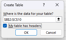
2. This will open the “Create Table” dialog box, where you will select your dataset and check the “My table has headers” box.

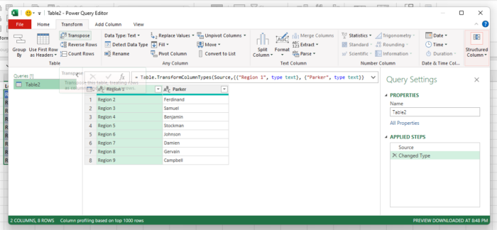
3. Now the “Power Query Editor” window will open, and then you will need to navigate to the “Transform” and select the “Transpose” option from within the “Table” group.

4. This will create a table in which your selected rows will now be converted into a single one.

As you can see, this method is extremely simple and does not require any familiarity working with formulas in Excel.

However, this will format the results as a table in order to transpose them into a single row.

You can change the formatting however you like once you have finished with the Power Query process.

Method #3 – Converting Multiple Rows Using the TEXTJOIN Function

Another function that can be used to convert multiple rows into one is the TEXTJOIN function.

With this function, we can join multiple rows into a single cell and separate them with a delimiter such as a comma.

This is simple to use and, in many cases, can make it easier to work with the data rather than working with multiple columns.

However, we will then show you how to separate the results into separate columns. The syntax for this function is:

=TextJoin(Delimiter, TRUE, Range)

The delimiter we will use in this case is a comma, and the TRUE simply instructs Excel to overlook empty cells.

Simply follow these steps to use TEXTJOIN to combine multiple rows.

1. Enter the TEXTJOIN formula into a blank cell where you would like the results to be located, and press Enter.

2. The TEXTJOIN function will take the range of rows and combine them into one cell separated by commas. In order to convert the results into their component values rather than the formula, select the cell, copy them, and then select “Paste Values” from the “Paste” dropdown on the ribbon.

3. Now you can separate the results by navigating to the “Data” tab, and from the “Data Tools” group, select the “Text to Columns” option.

4. This will open the “Convert Text to Columns Wizard.” In step 1 of the wizard, select Delimiter under “Choose the file type that best describes your data.”

5. In step 2, under “Delimiters,” select “Comma,” and in step 3, you will choose “Column data format,” which in most cases will be “General,” and select “Finish.”

6. Your data should now be neatly separated by a column.

This method is still relatively simple to use and offers the flexibility of merging your data into one cell, which can be useful in some circumstances.

Method #4 – Using the CONCATENATE Function To Convert Several Rows Into One

Excel is not lacking in functions, and another one that can be used to convert multiple rows into a single one is CONCATENATE.

This is a flexible function that, in our case, will work very similarly to TEXTJOIN.

Just like the previous function, CONCATENATE will combine all of our rows into one cell separated by a delimiter.

Just like with method number 3, we can use the Text to Columns tool from the ribbon to separate the results into multiple columns if desired.

The syntax for this function is:

CONCATENATE(text1, [text2], …)

It is important to keep in mind that though the CONCATENATE function is still available with backward compatibility, in Excel 2016 and newer, the function has been replaced by CONCAT.

However, for the most part, this newer function works extremely similarly, and the same steps below will similarly apply.

Here are the steps to follow to use the CONCATENATE function for converting multiple rows into one.

1. Enter the CONCATENATE function into an empty cell, including your cell references as the text separated by commas and quotation marks containing the delimiter you would like to use. In our case we will enter the formula =CONCATENATE(B2, “, “, B3, “, “, B4, “, “, B5, “, “, B6, “, “, B7, “, “, B8, “, “, B9, “, “, B10)

2. Once the formula is run, you should find the results separated by commas contained in the same cell. Copy the results and select “Paste Values” from the “Paste” dropdown on the ribbon to save the results as values rather than the formula.

3. Now follow steps 3 to 6 from Method #3 in order to use the “Text to Columns Wizard” to separate the results into distinct columns.

Now your results are all located on the same row but in separate columns. This method may not work in future versions of Excel using the CONCATENATE function. However, with few exceptions, the same techniques will apply using the newer CONCAT function.

Method #5 – Converting Multiple Rows Into One With the Ampersand Sign

You do not actually need to use any Excel text functions to get the job done when it comes to converting data from multiple rows into a single row.

You can actually combine multiple rows with nothing more than an ampersand sign.

To do this, you can simply join multiple rows of text by entering the cell references and ampersands to join them.

For example, =B2&” “&B3&” “&B4&” “&B5&” “&B6&” “&B7&” “&B8&” “&B9&” “&B10&” ” which is what we will use to join our regions.

Here is how to use the ampersand symbol to convert multiple rows into one.

1. Select the cell in which you would like the data to be placed.
2. Type = into the cell and then select the first cell. Follow this with an &, a quotation mark, a comma, a space, and then another quotation mark.

3. Repeat this procedure for each cell until you have a result like =B2&”, “&B3&”, “&B4&”, “&B5&”, “&B6&”, “&B7&”, “&B8&”, “&B9&”, “&B10&”” and then press “Enter.”
4. Now copy and paste the results as “Values” using the “Paste” dropdown.

5. Now repeat steps 3 to 6 from Method #3 in order to use the “Text to Columns Wizard” to separate the results into distinct columns.

This is a very simple solution that can still successfully combine multiple rows into a single one.

Conclusion

Oftentimes when working with a large amount of data, it can be easier to work with only a single row.

As you have seen, Excel provides numerous methods to convert multiple rows into just one, and this includes both ribbon tools and formulas, each of which can achieve the same result.

No matter how you prefer to do it, these tools can make it extremely easy to get the job done, no matter how experienced you are in working with Excel.