How to Convert Dates to Months and/or Years in Spreadsheet3 Basic Steps!

Last Updated: February 9, 2023

In Excel, date automatically adapts to the date cell whenever you type/enter a certain date in the cell you are typing in.

Excel recognizes the date inputs that you are typing – whether it is the day, month, or year.

This can be very beneficial in a lot of ways depending on the display format you want it to be shown in Excel.

It can even let you choose the parts of a certain date that you want to use, depending on your needs.

For instance, you only need the month and year format in your project, and the day part is not needed or irrelevant to the project. You can simply take out the day part of the date.

Now, Excel already recognizes what format you need in your project.

You may easily remove the day part and just extract the month and year part of the date by simply choosing the format you want to display on your work.

There are three ways in which you are able to change/convert date to month and year in Excel. This tutorial tackles how we can do this easily.

The Sample Data

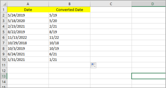
In this Excel tutorial, the following data set will be used as shown in the picture below.

The set of dates will be used to convert into months and years.

In every country, there are different date formats used.

It is important that we know the standard date format in that certain country that we are working in so we can work easily and efficiently.

In our example, in the US, the standard date format arrangement is month followed by the day, then lastly followed by the year (mm/dd/yyyy).

In other countries like the UK, the format of the date is day followed by the month and lastly followed by the year (dd/mm/yyyy). Other countries like Korea, China, and Iran use the formate opposite to that of the UK (yyyy/mm/dd).

Usually, Excel will depend on the date format of your computer’s settings.

The date format may differ from what you are currently working on, so make sure that the date format you are typing is in the correct order.

For instance, you want your date 2/10 to be October 2, but instead, the date is registered as February 10.

Dates to Months and/ or Years Conversion By MONTH and YEAR Function

In Excel, there are functions called the MONTH and YEAR functions. You can input and extract the month or year from a certain date for a date cell.

This must be done on a valid Excel date or else the function will have a #VALUE error result on the cell.

Below is the step-by-step process on how we can extract the month on our given sample date data mentioned earlier:

Select the blank cell (B2) where you like to place the month.
Input: =MONTH, followed by typing open parenthesis “(“.
Select the original date which contains the first cell (A2).
Then follow it by typing the close parenthesis “)”.
Hit the Enter Key.
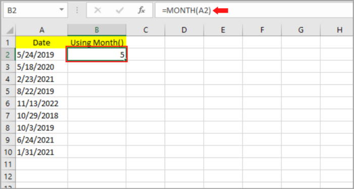
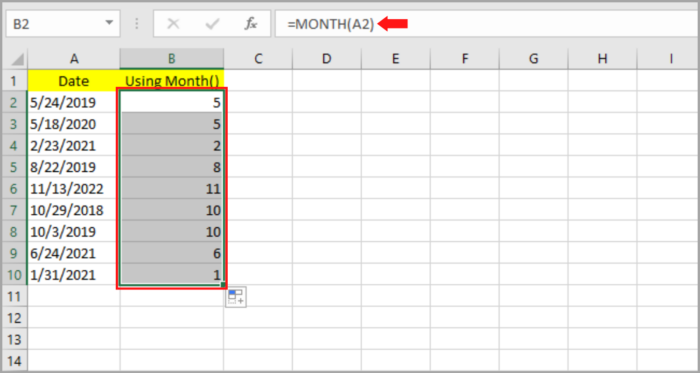
The month should be shown on the cell that you selected matching the original date. By dragging the fill handle downward or by clicking twice, you can copy this to the rest of the cell.

As you can see, column B is now filled with the month corresponding to the original date on column A.

At this point, we are about to learn how to take out the year from our previous example datum:

Select the blank cell (C2) where you like to place the month.
Input: =YEAR, followed by typing open parenthesis “(“.
Select the original date which contains the first cell (A2).
Then follow it by typing the close parenthesis “)”.
Hit the Enter Key.
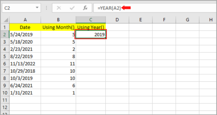
The month should be shown on the cell that you selected matching the original date. By dragging the fill handle downward or by clicking twice, you can copy this to the rest of the cell.

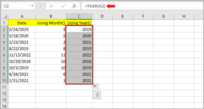
As you can see, column C is now filled with the year of the date corresponding to the original date on column A.

But what if we prefer to mix the two functions to show the months and years at the same time, following our desired format?

Assuming, “5-2019” is your preferred result and format for the date “5/24/2019” and you also want the same format for the rest of the cells.

Select the blank cell (D2) where you like to place the resulting date.
Input: =B2 & “-” & C2 or you may input: =MONTH(A2) & “-” & YEAR(A2).
Hit the Enter Key.
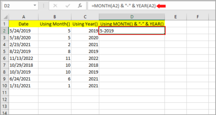
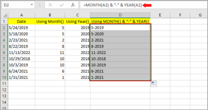
The month should be shown on the cell that you selected matching the original date. By dragging the fill handle downward or by clicking twice, you can copy this to the rest of the cell.

As you can see, column D2 is now filled with your preferred date format corresponding to the original date on column A:

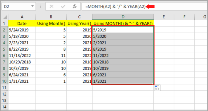
However, if you do not prefer a dash as the date separator “-” and instead you want the slash symbol “/”, then simply replace the dash with the slash sign at the formula bar.

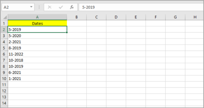
Lastly, if you want to remove the initial cell references you created and just want to leave the final formatted dates, you just have to make the final values as constants.

To do this, duplicate Column D by copying and pasting. Note: To paste the values only, right-click on the cell(s) and a pop-up menu will appear.

From the list, choose Paste Options then Values. You are now free to remove Column A to Column C and just have the preferred month-year date values as your dataset content.

Despite the simplicity of this method to modify dates, it is still unfamiliar to many.

This is because it fails to give much of a user’s flexibility in comparison with the two following methods we are going to illustrate in the next sections below.

Dates to Months and Years Conversion By TEXT Function

We use Excel’s TEXT function to transform number figures into values in letter format.

The TEXT function formula is:

= TEXT(value, format_code)

In the above formula,

the value indicates the number value or the cell reference to convert.
format_code indicates the conversion format.

The TEXT function will automatically register your designated values to the format_code and result in text values having a specified format.

Suppose that you have “5/24/2019” as your Cell A2, applying =TEXT(A2, “mm/yyyy”) as your formula will give “05/2019” as a result.

Below are several format codes that you can use.

Year Format Code Representations

To denote year values, apply the next two fundamental format codes:

yy – year abbreviation in two numbers such as 20 or 19
yyyy– year abbreviation in four numbers such as 2020 or 2019

Therefore:

when you input =TEXT(A2, yy) in our data date set illustration, it will then enter “19”.
when you input =TEXT(A2, yyyy), it will then enter “2019”.

Months of the Year Format Code Representations

To denote month values, apply the next four fundamental format codes:

m – month abbreviation in a non-zero numeral/s such as 5 or 10
mm – month abbreviation in exact two numerals such as 05 or 10
mmm – month abbreviation in three letters such as Aug or Dec
mmmm – complete month’s name such as May or February

Therefore:

when you input =TEXT(A2, mm) in our data date set illustration, it will result in “12”.
when you input =TEXT(A2, mmm), it will result in “Dec”.
when you input =TEXT(A2, mmmm), it will result in “December”.

Next, Let’s find out how the TEXT function works in converting all the Column A dates into various formats in our set of values:

The following is the step-by-step process on how we can extract the month and year on our given sample date data by applying the function of TEXT:

Select the blank cell (B2) where you like to place the date result.
Input: =TEXT(A2,”m/yy”).
Hit the Enter Key.
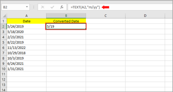
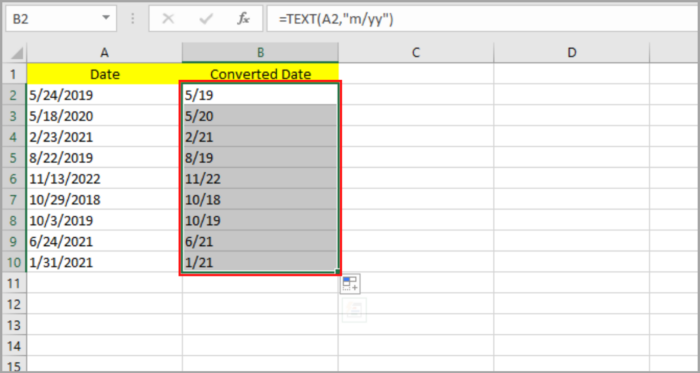
The month/year should be shown on the cell that you selected matching the original date. By dragging the fill handle downward or by clicking twice, you can copy this to the rest of the cell.

Lastly, if you want to remove the initial cell references you created and just want to leave the final formatted dates, you just have to make the final values as constants.

To do this, duplicate Column B by copying and pasting. Note: To paste values only, right-click on the cell and a pop-up menu will appear.

From the list, choose Paste Options then Values. You are now free to remove Column A and just have the preferred month/year date values as your dataset content.

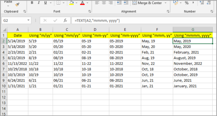
The code of your input value format will change (at step 2) depending on your preferred month-year format.

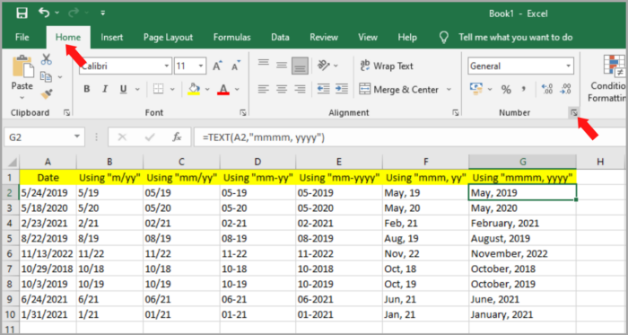
Below are the codes and their corresponding results when used in Cell A2:

when you input =TEXT(A2, “mm/yy”) in our set of values illustration, it will result in “05/19”.
when you input =TEXT(A2, “mm-yy”) in our set of values illustration, it will result in “05-19”.
when you input =TEXT(A2, “mm-yyyy”) in our set of values illustration, it will result in “05-2019”.
when you input =TEXT(A2, “mmm/yy”) in our set of values illustration, it will result in “May,19”.
when you input =TEXT(A2, “mmmm/yyyy”) in our set of values illustration, it will result in “May, 2019”.

Thus, the TEXT function can be applied when converting dates to any user’s preferred format. Just simply modify the code based on your preference or format requirement.

Important Note: With the use of the previously mentioned formulas, your date values will instantly change into text format. So, if in case, you like to revert the format, just use the Format Cell dialog box.

Dates to Months and Years Conversion By Number Format

Format Cell is one of Excel’s multifunctional features that ease users’ formatting experience through a categorized dialog box.

Below is an illustration of how to do date conversions using our set of data in several formats.

Pick the date cells you prefer to format (A2:A10).
On your mouse, hit the right button. A dialog box will pop up. Choose Format Cells. Or, Under the Home Menu, go to the Number group and select the diagonal arrow at the bottom right.
As the dialog box appears, go to Number Tab.
At the left side of the dialog box, you will find the category, choose ‘Date’.
Several number formatting selections will appear on the right side of the box.
Choose your preferred format. For instance, to show the date in the format “May-19”, subsequently, pick the corresponding date formatting template.
In case your preferred format is not on the listed date formats, don’t worry. You can select ‘Custom’ under the Category list. This serves as a cell-custom-format converter.
Check first if your desired format is listed in the templates under ‘Type’. Else ways, just input the codes in the box under ‘Type’. Hence, input “m/yy” at the box to format the initial month as “5/29”.
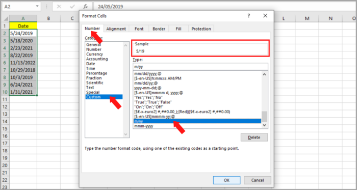
Select the OK button.

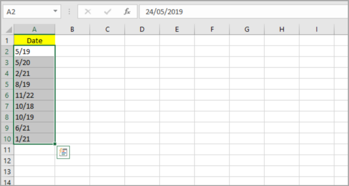
At this point in time, you should already convert all the date cells into the desired format.

Compared to the earlier method, by TEXT function, the last method varies in four different aspects:

Using the last method, you can now apply the function right onto the first cells.
You can now convert in a snap. No more hassle of adding other cells for formula input and pasting the values right after and, in the end, you will just delete the initial cells, as necessary, if you are using the function TEXT.
This feature only varies the date’s format and keeps the original date values. Therefore, if you prefer to revert the date values, you can simply do it. Note: By using the function TEXT, the first dates will be lost due to the variation of the whole datum.
With this function, you will get date formatted results instead of text, with no conversion needed, you can do formatting straight ahead.

Now, we learned the three easy ways to format dates to months and/or years in an Excel spreadsheet.

By following the step-by-step processes, we illustrated, you can now effortlessly change the dates in your required format.

We hope that this tutorial is easy to understand and helpful to you as you apply the steps in your dataset.